19.1 Trend and Seasonality

In general, trends in the data can be linear: \[y_t = \beta_0 + \beta_1 \cdot t + \epsilon_t\] or exponential: \[\ln(y_t) = \beta_0 + \beta_1 \cdot t + \epsilon_t\] Note that \(\beta_1\) in the exponential time trend model is the average annual growth rate (assuming \(t\) is in years). Often, data can be decomposed into three components:

Trend
Season
Random component

The seasonal component can be included via dummy variables. For example, for quarterly data the following model can be used:

\[y_t=\beta_0+\delta_1 \cdot Q1_t+\delta_2 \cdot Q2_t+\delta_3 \cdot Q3_t+\beta_1 \cdot x_{1,t}+ \cdots+\beta_k \cdot x_{k,t}+\epsilon_t\] One seasonal dummy must be dropped. That is, quarterly and yearly data require three and eleven dummy variables, respectively. Consider the retail data.

retail$date  = as.Date(retail$date,format="%Y-%m-%d")
retail$month = format(retail$date,"%m")
retail$t     = c(1:nrow(retail))
bhat         = lm(retail~factor(month)+t,data=retail)
retail$fit   = predict.lm(bhat)
ggplot(retail)+
  geom_line(mapping=aes(x=date,y=retail),color="red")+
  geom_line(mapping=aes(x=date,y=fit))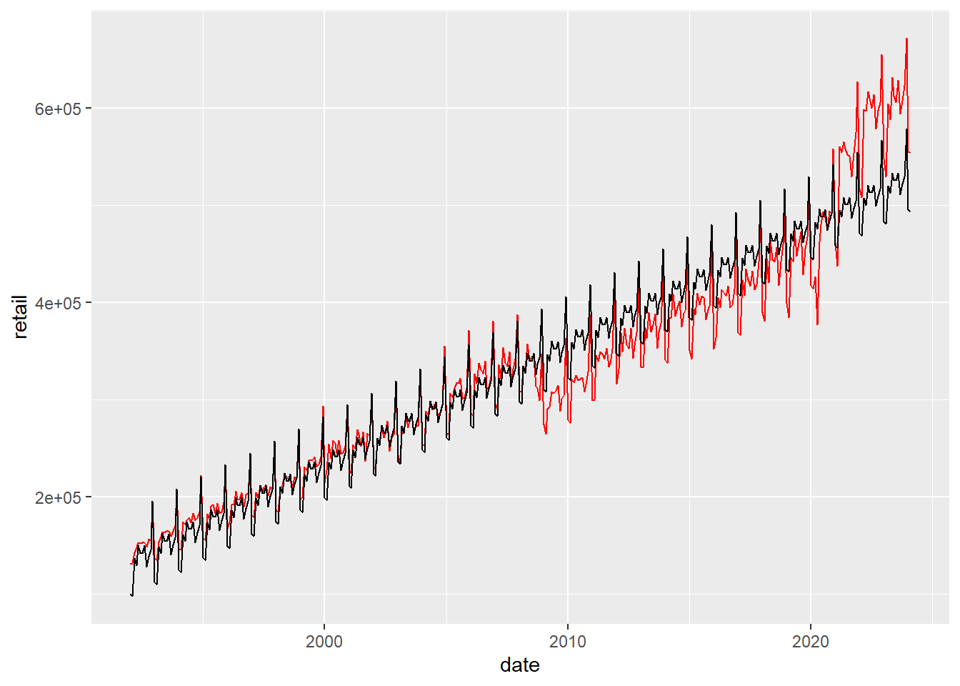

A second example considers quarterly beer production in Australia. In a first step, the data is converted into a time series:

beer = ts(beer$production,start=c(1992,1),end=c(2014,4),frequency=4)

Next, the data is plotted using a function from the package ggfortify. Additional documentation using the package is found under Plotting ts objects.

autoplot(beer)

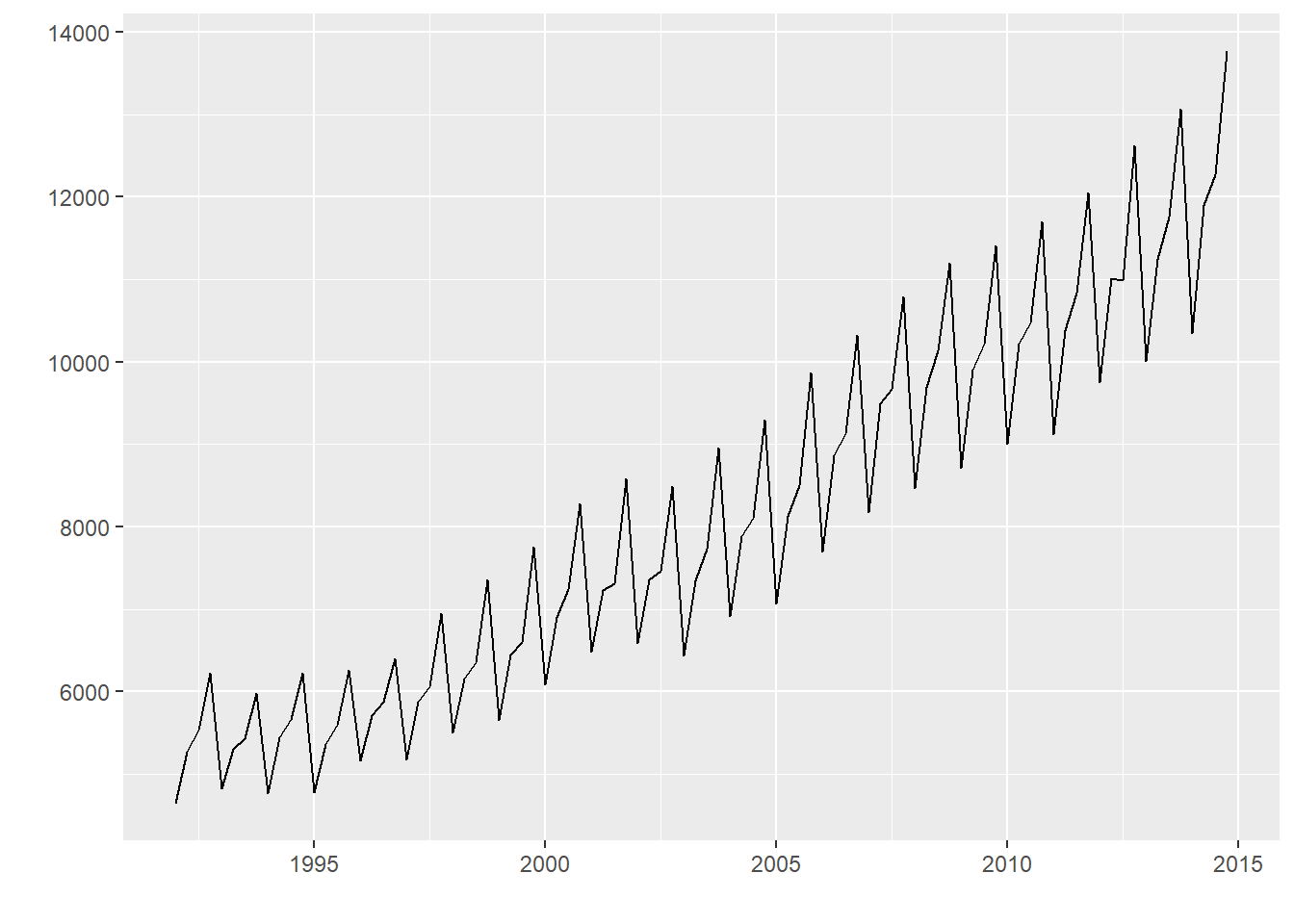
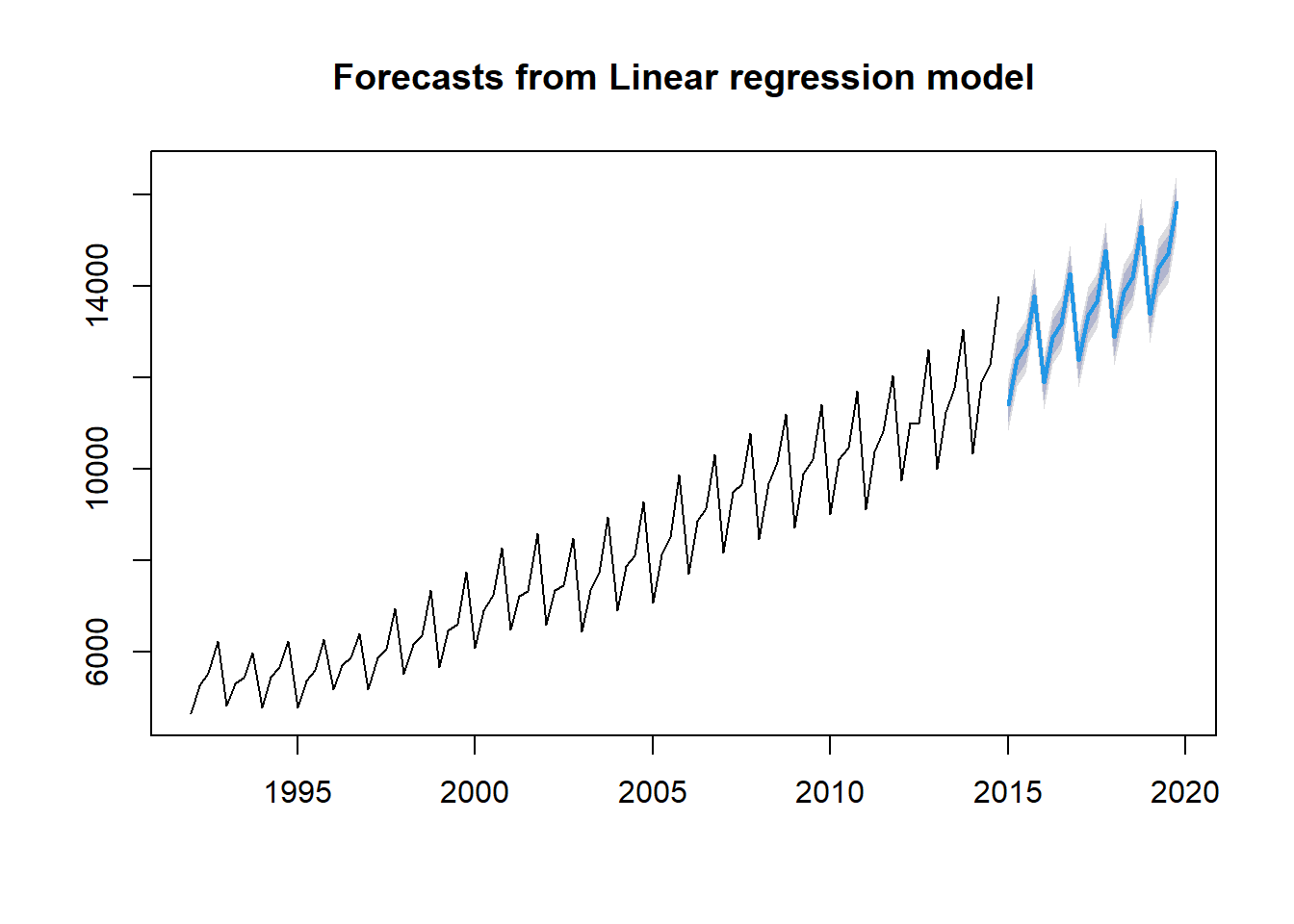
Note that the beer now appears in a different category in the Global Environment, i.e., not under “Data” anymore. The function tslm from the package forecast is used next. The function fits a linear model including seasonality and a trend component (and a trend-squared component if desired).

bhat = tslm(beer~trend+I(trend^2)+season)
summary(bhat)

## 
## Call:
## tslm(formula = beer ~ trend + I(trend^2) + season)
## 
## Residuals:
##     Min      1Q  Median      3Q     Max 
## -677.24 -163.84    2.12  195.34  529.37 
## 
## Coefficients:
##              Estimate Std. Error t value Pr(>|t|)    
## (Intercept) 4.082e+03  9.865e+01  41.381  < 2e-16 ***
## trend       3.975e+01  4.298e+00   9.249 1.53e-14 ***
## I(trend^2)  4.200e-01  4.477e-02   9.381 8.26e-15 ***
## season2     8.677e+02  7.987e+01  10.864  < 2e-16 ***
## season3     1.043e+03  7.990e+01  13.061  < 2e-16 ***
## season4     2.031e+03  7.993e+01  25.408  < 2e-16 ***
## ---
## Signif. codes:  0 '***' 0.001 '**' 0.01 '*' 0.05 '.' 0.1 ' ' 1
## 
## Residual standard error: 270.8 on 86 degrees of freedom
## Multiple R-squared:  0.9867, Adjusted R-squared:  0.9859 
## F-statistic:  1278 on 5 and 86 DF,  p-value: < 2.2e-16

The package forecast can be also be used to forcast:

plot(forecast(bhat,h=20))

19.1.1 Practice Exercise

Consider the data in ez. It contains unemployment claims (\(uclms\)) from Anderson (IN) before and after the establishments of an enterprise zone (EZ). The purpose of an EZ is to provide incentives for business to invest in area that are usually plagued by economic distress. Execute two regression models with \(\ln(uclms)\) as the dependent variable and including a time trend and monthly dummy variables as the independent variables: (1) without \(EZ\) and (2) with \(EZ\). What can be concluded in terms of trend, seasonality, and the effectiveness of the EZ.
Consider the data in traffic which contains information on accidents, traffic laws, and other variables for California. The dependent variable of interest is the natural log of \(totacc\). In a first regression, use the time trend and monthly dummy variables as the independent variables. In a second regression, add \(wkends\), \(unem\), \(spdlaw\), and \(beltlaw\). What can be concluded in terms of trend, seasonality, and the effectiveness of the laws concerning speed limits and belt usage. Why would weekends and unemployment be important?