6.2 Discrete Probability Distributions
A random variable \(X\) is said to be discrete if it can assume only a finite or countable infinite number of distinct values. A discrete random variable can be defined on both a countable or uncountable sample space. The probability that \(X\) takes on the value \(k\), i.e., \(P(X=k)\), is defined as the sum of the probabilities of all sample points that are assigned the value k. For each value within its domain, we have \(P(X=k) \geq 0\) and that the sum of all probabilities is equal to one. For example, suppose you are flipping a coin three times and associate the outcome “heads” with the number one. The results of this experiment are illustrated in the table below.
| Outcome | HHH | HHT | HTH | HTT | THH | THT | TTH | TTT |
|---|---|---|---|---|---|---|---|---|
| Pr | 1/8 | 1/8 | 1/8 | 1/8 | 1/8 | 1/8 | 1/8 | 1/8 |
| X | 3 | 2 | 2 | 1 | 2 | 1 | 1 | 0 |
This experiment can also be represented with a histogram which can be turned into a frequency histogram. This is illustrated for tossing a coin ten times and repeating the experiment 10,000 times.
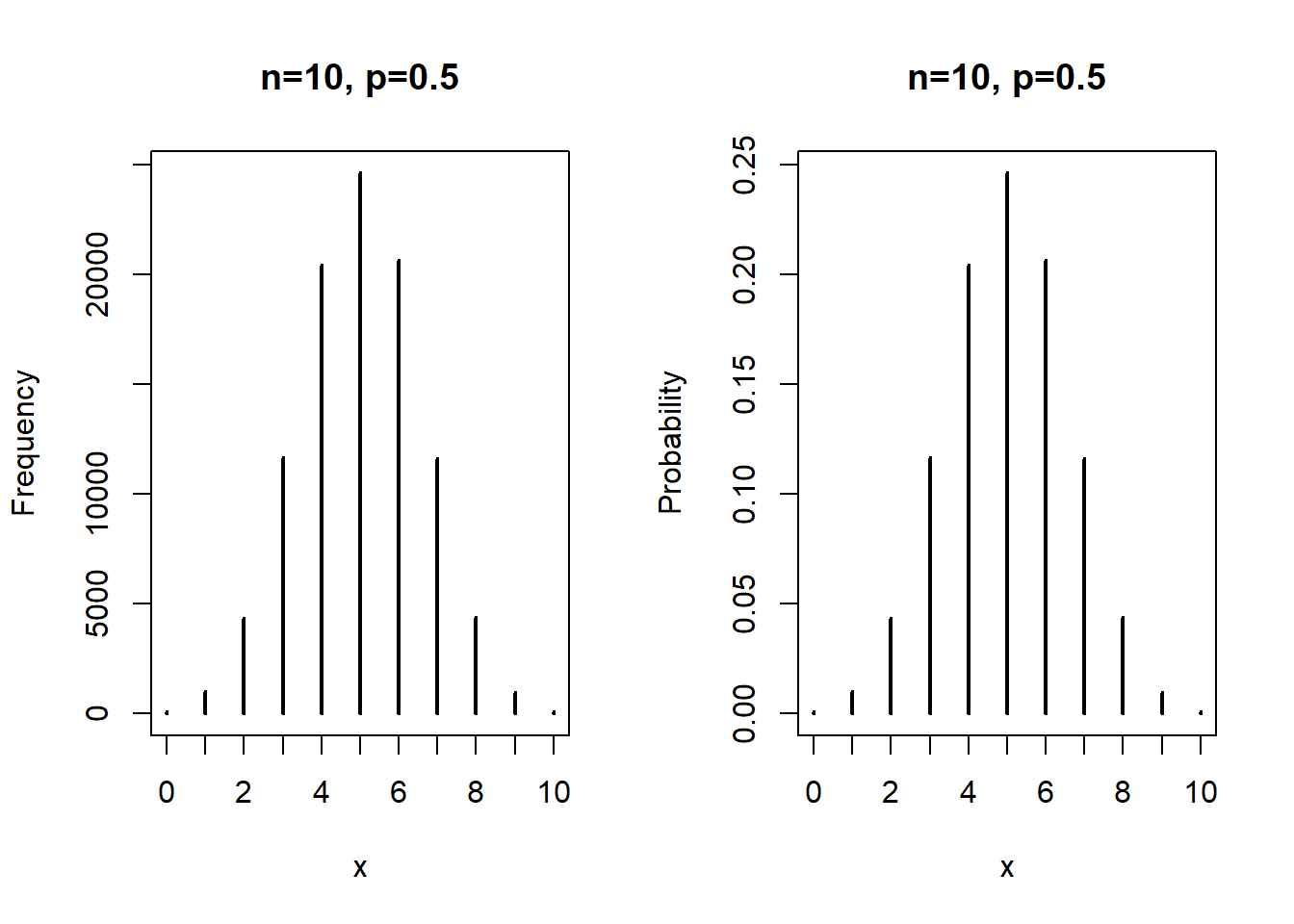
Figure 6.1: Tossing a coin ten times and repeating the experiment 1000 times.
6.2.1 Bernoulli distribution
The Bernoulli (named after Jacob Bernoulli, 1654-1705) distribution is the simplest probability distribution. There are only two outcomes: Success and Failure. The distribution is characterized by one parameter, i.e., \(p\). The probability mass function is written as \(P(X=1)=p\) and, correspondingly, \(P(X=0)=1-p\). The expected value of the binomial is written as follows: \[E(x)=1 \cdot p+0 \cdot (1-p)=p\] To calculate the variance, we have \(E(x^2)=1^2 \cdot p + 0^2 \cdot (1-p)=p\) and \(E(x)^2=p^2\). Thus, we have \[Var(x)=E(x^2)-E(x)^2=p\cdot(1-p)\]
6.2.2 Binomial distribution
The binomial distribution is closely related to the Bernoulli distribution because it represents repeated Bernoulli outcomes. The two parameters are \(n\) and \(p\). The number of successes is represented by \(k\). The probability mass function is written as \[Pr(X=k) = {n \choose k} \cdot p^k \cdot (1-p)^{n-k}\] The expected value of \(X\) is \(E(X)=n \cdot p\) and the variance is \(Var = n \cdot p \cdot (1-p)\). A situation must meet the following conditions for a random variable \(X\) to have a binomial distribution:
- You have a fixed number of trials involving a random process; let \(n\) be the number of trials.
- You can classify the outcome of each trial into one of two groups: success or failure.
- The probability of success is the same for each trial. Let \(p\) be the probability of success, which means \(1-p\) is the probability of failure.
- The trials are independent, meaning the outcome of one trial does not influence the outcome of any other trial.
Imagine a multiple choice test with three questions and five choices for each question. First, draw a probability tree. What is the probability of two correct responses? Next, the binomial distribution is used to calculate the probability. \[P(X=2) = {3 \choose 2} \cdot 0.2^2 \cdot (1-0.2)^{3-2} =0.096\] and \[P(X=3) = {3 \choose 3} \cdot 0.2^3 \cdot (1-0.2)^{3-3} =0.008\] Summing up both probabilities gives us \(P(X \ge 2) = 0.104\).
The binomial distribution can be used to analyze the issue of overbooking. Assume that an airline as a plane with a seating capacity of 115. The ticket price for each traveler is $400. The airline can overbook the flight, i.e., selling more than 115 tickets, but has to pay $700 in case a person has a valid ticket but needs to be re-booked to another flight. There is a probability of 10% that a booked passenger does not show up. The results for overbooking between 1 and 31 seats are shown in the figure below.
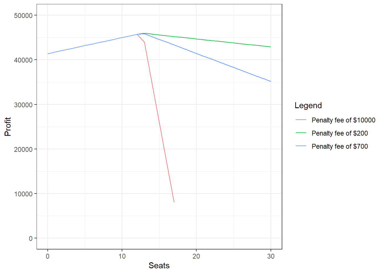
Figure 6.2: Example of using the binomial distribution to determine how many seats to sell over capacity.
6.2.3 Poisson Distribution
The Poisson distribution is used for count data (i.e., \(0,1,2,...\)). The probability mass function for the Poisson distribution is given by the following equation: \[P(X=k)=\frac{\lambda^k \cdot e^{-\lambda}}{k!}\] An example of the Poisson distribution (named after Simeon Denis Poisson, 1781-1840) for different parameter values is shown below.
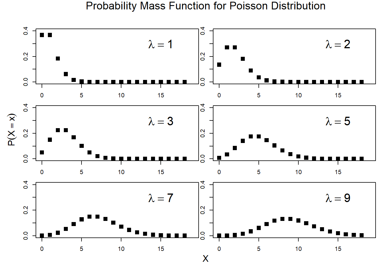
Figure 6.3: Poisson Distribution