16.1 Ordered Logit Model
Suppose that respondents are asked if they are going to get a COVID-19 vaccine. The choices are
- Definitely yes
- Probably yes
- Probably no
- Definitely no
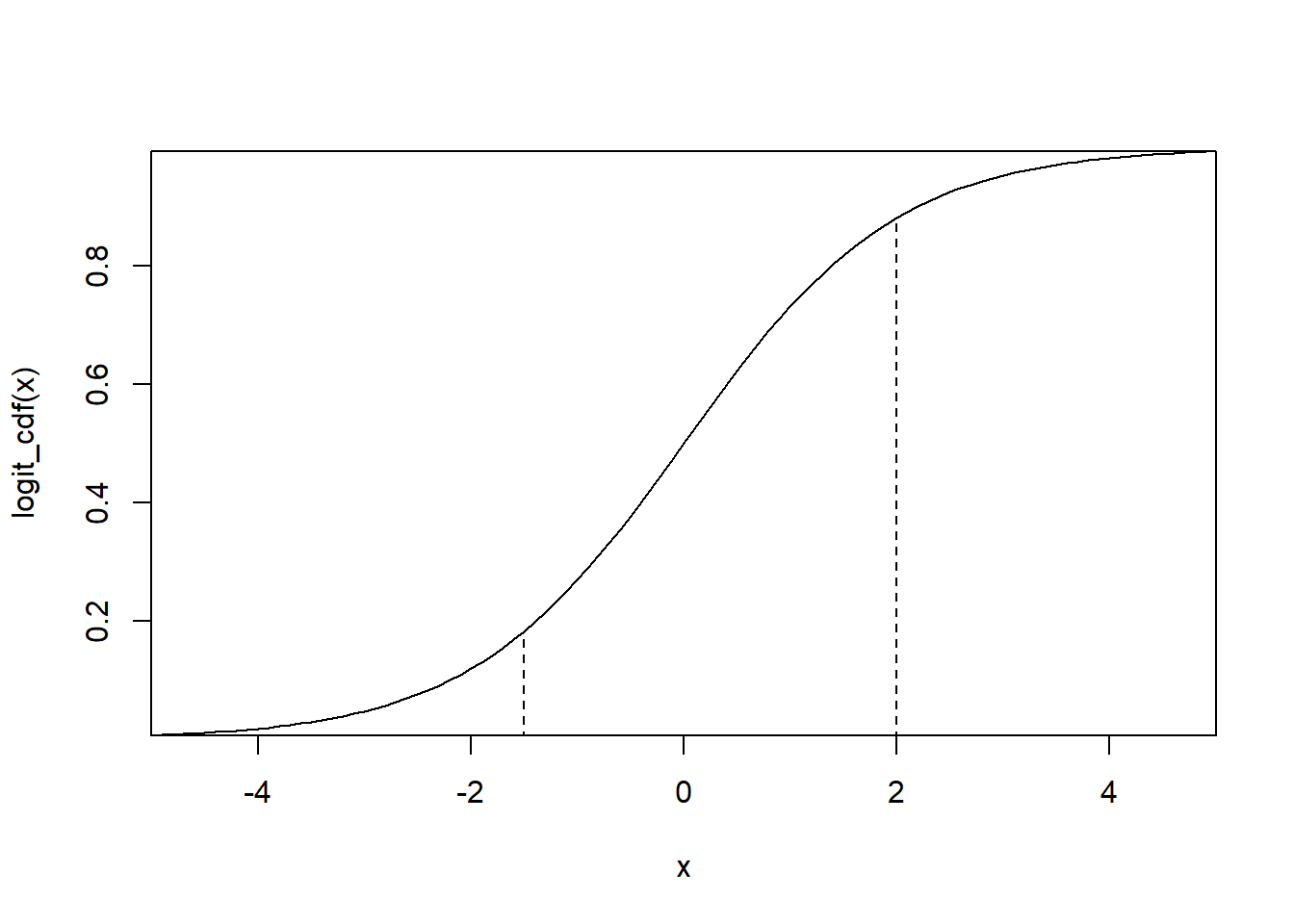
The ordered logit model assumes the presence of a latent (unobserved by the researcher) variable \(y^*\): \[y_i^* = \beta_0+\beta_1 \cdot x_i + \epsilon_i\] In the case of the vaccine model, this may be a measure of trust in vaccines. What the researcher does measure is an \(m\)-alternative ordered model: \[y_i = j \quad \text{if} \quad \alpha_{j-1} < y_i^* \leq \alpha_j \quad \text{for} \quad j=1, \dots,m\] where \(\alpha_0 = - \infty\) and \(\alpha_m=\infty\). In this case, we have \[ \begin{aligned} Pr(y = j) &=Pr(\alpha_{j-1} < y_i^* \leq \alpha_j)\\ &=Pr(\alpha_{j-1} < \beta_0+\beta_1 \cdot x_i + \epsilon_i \leq \alpha_j)\\ &=Pr(\alpha_{j-1}- \beta_0-\beta_1 \cdot x_i < \epsilon_i \leq \alpha_j - \beta_0-\beta_1 \cdot x_i)\\ &=F(\alpha_j - \beta_0-\beta_1 \cdot x_i)-F(\alpha_{j-1} - \beta_0-\beta_1 \cdot x_i) \end{aligned} \] For the ordered logit: \(F(z)=exp(z)/(1+exp(z))\). The cut-off example points for the graph below are \(\alpha_0 = -\infty\), \(\alpha_2 = -1.5\), \(\alpha_3 = 2\), and \(\alpha_4 = \infty\)
16.1.1 Ordered Logit Example: Organic Food Purchase
The order logit model is illustrated with a survey on the purchase frequency of organic tomatoes and organic strawberries fpdata:
- Never (1), rarely (2), once per month (3), every 2 weeks (4), 1-2 times a week (5), almost daily (6)
The independent variables included in the model are
- Age and female
- Education: High school (1), some college (2), bachelor (3), master (4), technical school diploma (5), doctorate (6)
fpdata$strawberriesorg = as.factor(fpdata$strawberriesorg)
strawdata = fpdata[c("strawberriesorg","age","education","female","kidsunder12")]
strawdata = na.omit(strawdata)
bhat = polr(strawberriesorg~age+education+female+kidsunder12,data=strawdata,Hess=TRUE)
summary(bhat)
## Call:
## polr(formula = strawberriesorg ~ age + education + female + kidsunder12,
## data = strawdata, Hess = TRUE)
##
## Coefficients:
## Value Std. Error t value
## age -0.02034 0.009838 -2.0676
## education 0.01596 0.112028 0.1425
## female -0.41533 0.280485 -1.4808
## kidsunder12 0.28560 0.321778 0.8876
##
## Intercepts:
## Value Std. Error t value
## 0|1 -1.4958 0.6497 -2.3022
## 1|2 -0.4381 0.6434 -0.6810
## 2|3 0.2084 0.6394 0.3259
## 3|4 0.8352 0.6442 1.2964
## 4|5 1.6314 0.6699 2.4353
##
## Residual Deviance: 526.4547
## AIC: 544.4547For the organic purchases data, the cut-off points are under “Intercepts” and thus, we have (rounded coefficients): \[z = -0.020 \cdot age +0.0160 \cdot education -0.415 \cdot female +0.286 \cdot kidsunder12\] The cut-off points can be interpreted as follows: \[ \begin{aligned} Pr(y=1) &= P(z+\epsilon_i \leq -1.4958)\\ Pr(y=2) &= P(-1.4958 < z+\epsilon_i \leq -0.4381)\\ Pr(y=3) &= P(-0.4381 < z+\epsilon_i \leq 0.2084)\\ Pr(y=4) &= P(0.2084 < z+\epsilon_i \leq 0.8352)\\ Pr(y=4) &= P(0.8352 < z+\epsilon_i \leq 1.6314)\\ Pr(y=6) &= P(1.6314 \leq z+\epsilon_i ) \end{aligned} \] In order to get the \(p\)-values displayed in the output, you have to execute two additional steps:
bhat.coef = data.frame(coef(summary(bhat)))
bhat.coef$pval = round((pnorm(abs(bhat.coef$t.value),lower.tail=FALSE)*2),2)
bhat.coef
## Value Std..Error t.value pval
## age -0.02034185 0.009838336 -2.0676110 0.04
## education 0.01595914 0.112027882 0.1424569 0.89
## female -0.41533145 0.280485372 -1.4807598 0.14
## kidsunder12 0.28560319 0.321777883 0.8875787 0.37
## 0|1 -1.49575271 0.649708891 -2.3021891 0.02
## 1|2 -0.43813109 0.643390358 -0.6809724 0.50
## 2|3 0.20839939 0.639383205 0.3259382 0.74
## 3|4 0.83515493 0.644195302 1.2964313 0.19
## 4|5 1.63135404 0.669870994 2.4353257 0.0116.1.2 Predicted Probability and Marginal Effects
The predicted probability for each observation can be obtained as well assuming that the output of the polr command is stored in \(bhat\).
##             effect.0 effect.1 effect.2 effect.3 effect.4 effect.5
## age            0.005    0.000   -0.001   -0.001   -0.001   -0.001
## education     -0.004    0.000    0.001    0.001    0.001    0.001
## female         0.098   -0.003   -0.023   -0.024   -0.023   -0.026
## kidsunder12   -0.067    0.001    0.015    0.017    0.016    0.018