6.3 Continuous distributions

We define a random variable to be continuous if \(F_X(x)\) is a continuous function of \(x\) and for every real number \(x\). The probability density function, \(f_X(x)\), of a continuous random variable X is the function \(f(\cdot)\) that satisfies \[F_X(x)=\int_{-\infty }^{x} f_{X}(u) du\] Properties are that \(f_X(x) \geq 0\) for all \(x\) and \[ \int_{-\infty }^{\infty } f_X(x) dx =1\] It is important to note that for a continuous distribution, the probability of a particular event is zero.

6.3.1 Uniform distribution

The simplest continuous distribution is the uniform distribution. If \(a<b\), a random variable \(X\) is said to have a uniform probability distribution on the interval \((a,b)\) if and only if the density function of \(X\) is \[f(x) = \frac{1}{b-a}\] Parameters defining a uniform distribution: \(a,b\). Suppose that a package is scheduled to be delivered between 9:00 (9am) and 20:00 (8pm). You are out for lunch between 12:00 (noon) and 13:30 (1:30pm). The probability that the package arrives during the lunch break is \(P(12<x<13)=\frac{1}{20-9} \cdot 1.5 \approx 13.64\%\).

6.3.2 Normal distribution

The random variable \(X\) is said to be normally distributed with mean \(\mu\) and variance \(\sigma^2\) (abbreviated by \(x \sim N[\mu,\sigma^2\)) if the density function of \(x\) is given by \[f(x;\mu,\sigma^2)=\frac{1}{\sqrt{2\pi \sigma^2}}\cdot e^{{\frac{-1}{~2} \left(\frac{x-\mu}{\sigma}\right)}^2}\] The Normal distribution can be derived from the Binomial Distribution.

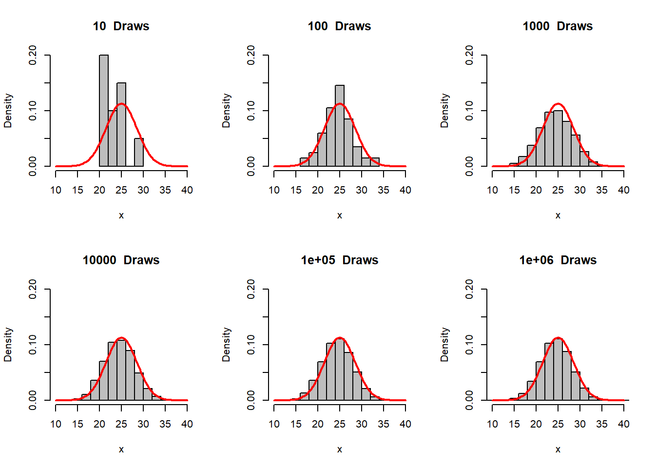
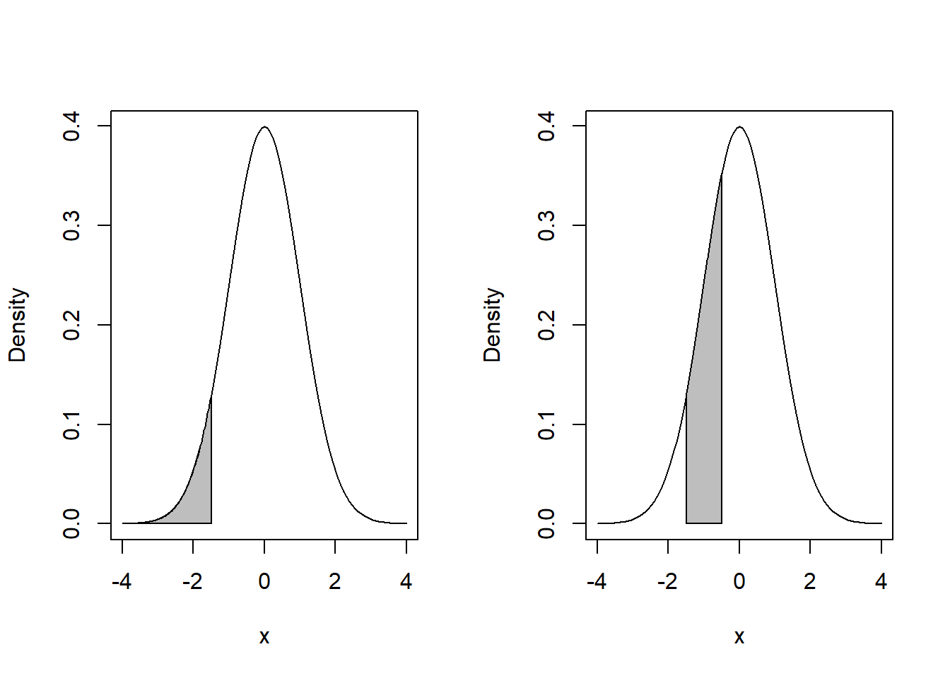
The normal probability density function is bell-shaped and symmetric as shown in the figure. It is usually necessary to standardize the normal distribution to make it N(0,1): \[z = \frac{X-\mu}{\sigma}\] where \(z\) is the distance from the mean of a Normal distribution expressed in units of the standard deviation. Suppose that we have \(\mu = 75\) and \(\sigma = 10\) and we want to find \(P(x<60)\) and \(P(60<x<70)\). \[Pr(x<60) \Rightarrow \frac{60-75}{10}=-1.5\\ P(60<x<70) \Rightarrow z_1 = -1.5, z_2 = -0.5\] The normal distribution can be derived from the binomial distribution (Galton board). Assume that the average height of males and females in the U.S. is \(\mu_M=70\) and \(\mu_F=65\) inches, respectively. The standard deviations are \(\sigma_M=4\) and \(\sigma_F=3.5\). Calculate the probabilities associated with being \(\sigma\), \(2 \cdot \sigma\), and \(3 \cdot \sigma\) away from the mean. For more information on how the Normal Distribution evolved, see The Evolution of the Normal Distribution.

6.3.3 t-Distribution

Hence, we have to replace it with an estimate, i.e., with the value of the sample standard deviation. To calculate the Student \(t\) distribution, we need the degrees of freedom as well: \(t_{\alpha,\nu}\). This distribution was published by William Gosset in 1908. His employer, Guinness Breweries, required him to publish under a pseudonym, so he chose “Student”.

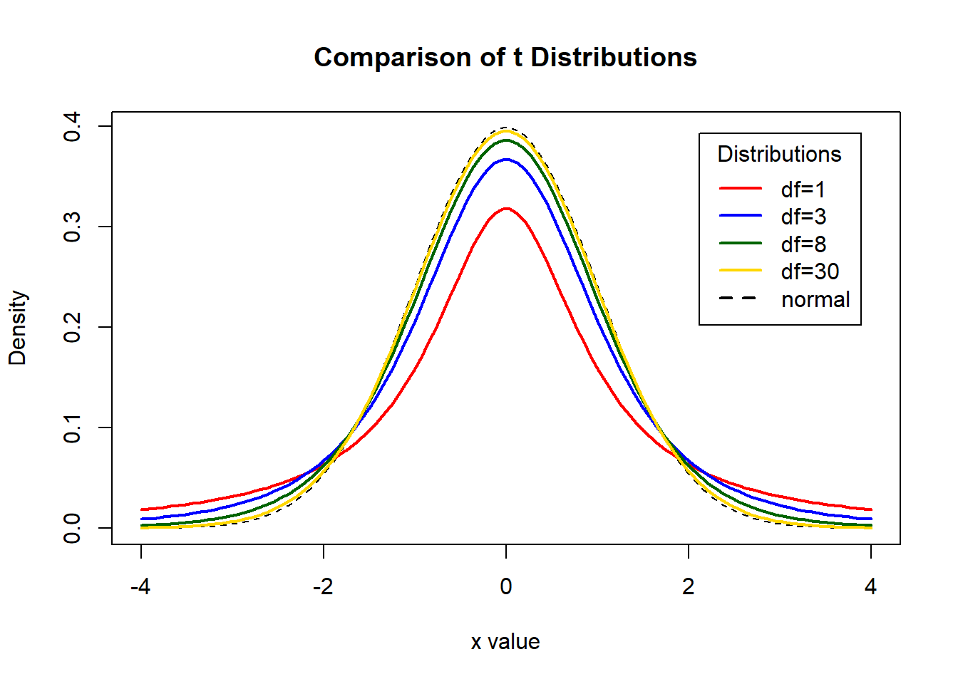
Figure 6.4: Student Distribution for various levels of degrees of freedom and Normal distribution