4.6 Covariance and Correlation Coefficicent
The previous sections focused on one random variable at a time. Very often, we have more two or more random variable and we are interested in their relationship. We will analyze the relationship between variables from a causal standpoint in the section on regression analysis. In this chapter, we focus on two variables and how they behave jointly. For now, we will not make any statements about causality. The important part here: Correlation is not causation! As for the variance, there are two definitions/equations to calculate the covariance between two variables: \[Cov(x,y)=E[(x-E(x))\cdot (y-E(y))]=E(x \cdot y)-E(x)E(y)\] If the sign of the covariance is positive, then \(x\) and \(y\) tend to move in the same direction, i.e., if one variable increases, the other variable increases as well. If the sign of the covariance is negative, then \(x\) and \(y\) tend to move in opposite directions, i.e., if one variable decreases, the other increases. If \(X\) and \(Y\) are independent, then \(Cov(X,Y)=0\). The covariance has several properties:
- Property 1: \(Var(X+Y)=Var(X)+Var(Y)+ 2 \cdot Cov(X,Y)\)
- Property 2 (Transformation of the covariance): \(Cov(r \cdot X+s,t \cdot Y+u)=r \cdot t \cdot Cov(X,Y)\)
The most important aspect about correlation (and statistics in general): Correlation does not mean causation. Causation requires a strong theoretical believe that one variable is the cause of another variable, e.g., influence of education on income. The correlation coefficient (sometimes called Pearson’s r) is defined as \[\rho(X,Y) = \frac{Cov(X,Y)}{\sqrt{Var(X) \cdot Var(Y)}}\] The correlation coefficient varies between \(-1\) and \(1\). The Sign provides the direction of the relationship between two variables and the Value provides the magnitude of the relationship. Note that the correlation coefficient has no dimensions!
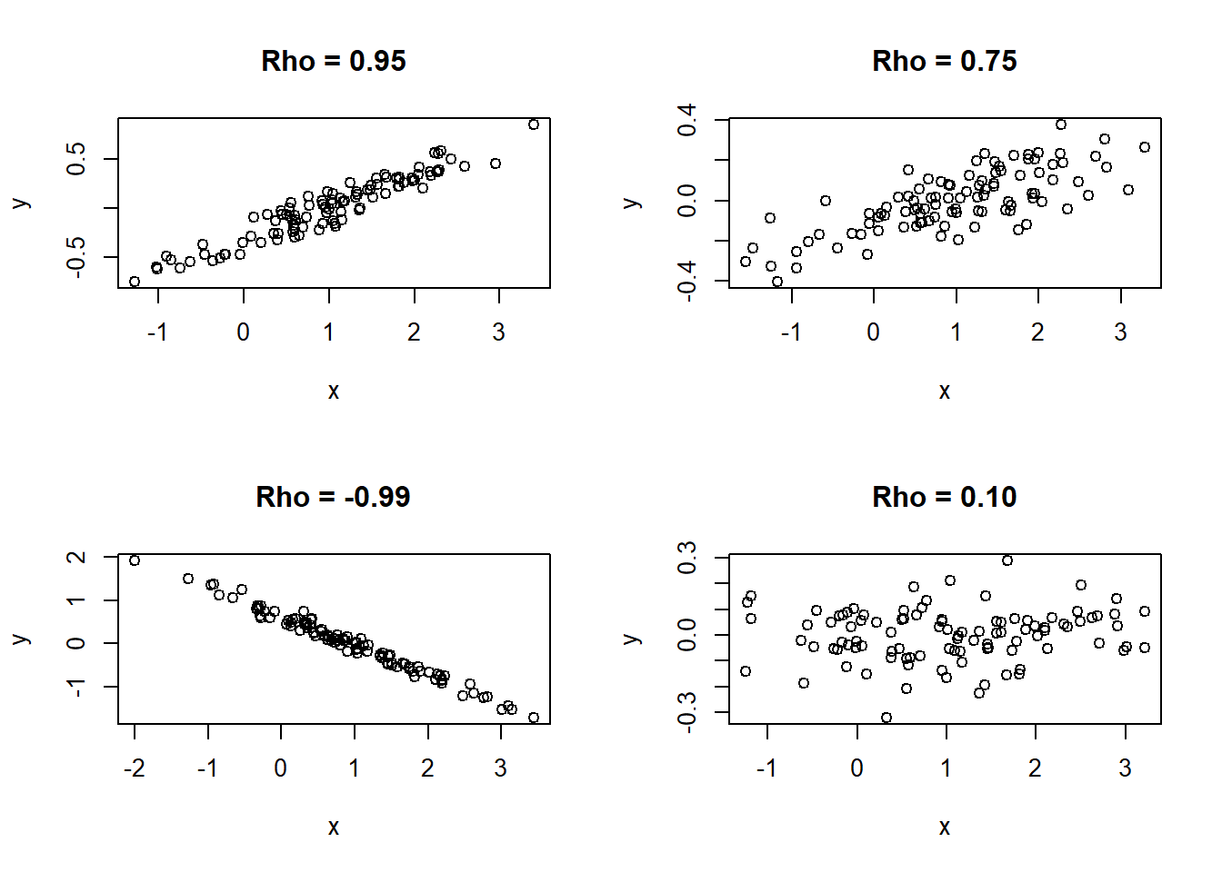
Figure 4.5: Examples of various correlation coefficients
A second example uses the data mh2 and the resulting scatter plot is shown below.
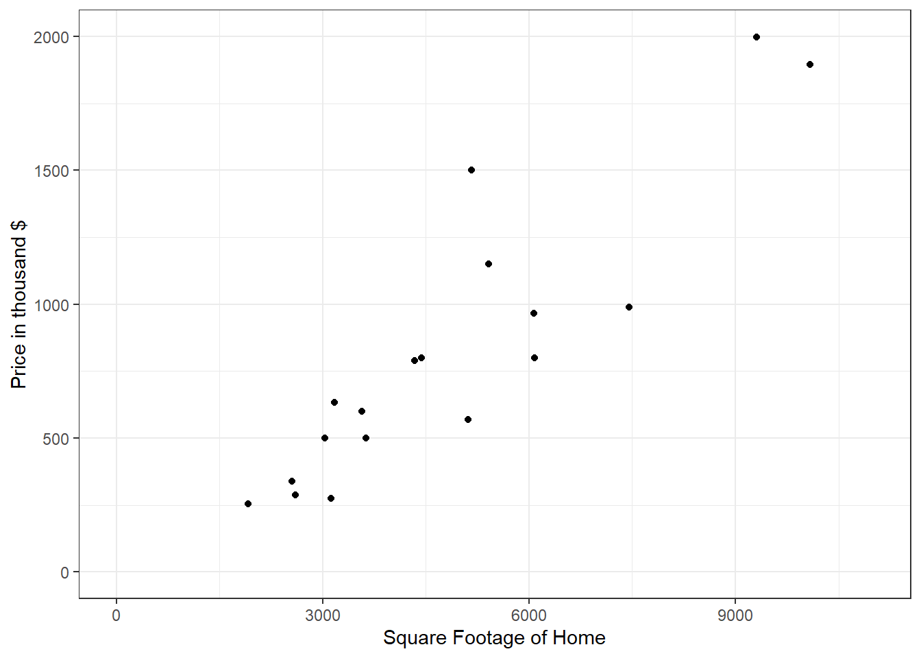
Figure 4.6: Correlation between the square footage of a home and the price of the home in the Meridian Hills neighborhood in Indianapolis.
The function summary() gives you mean, median, and quartiles for the eruption and waiting times. The functions var() and cor() calculate the variance, covariance, and correlation coefficient associated with the data sets. We will see in subsequent chapters how to interpret the covariance and correlation coefficients.
##    eruptions        waiting
##  Min.   :1.600   Min.   :43.0
##  1st Qu.:2.163   1st Qu.:58.0
##  Median :4.000   Median :76.0
##  Mean   :3.488   Mean   :70.9
##  3rd Qu.:4.454   3rd Qu.:82.0
## Max. :5.100 Max. :96.0## eruptions waiting
## eruptions 1.302728 13.97781
## waiting 13.977808 184.82331## [1] 0.9008112Note that sometimes, we deal with qualitative data, i.e., data that is not expressed as a number but as an expression. Example are gender (male/female), owning a car (yes/no), modes of commute (car, bike, train, bus, etc.). Consider the data in gssgun. One way to count the responses for firearm ownership is to use the following command:
table(gss$owngun)
Suppose you are only interested in people who answer yes or no for the questions concerning arrests and firearms ownership. You will have to subset the data.
##
##
##    Cell Contents
## |-------------------------|
## |                       N |
## |           N / Row Total |
## |           N / Col Total |
## |         N / Table Total |
## |-------------------------|
##
##
## Total Observations in Table:  2301
##
##
##              | df$sex
##    df$owngun |         1 |         2 | Row Total |
## -------------|-----------|-----------|-----------|
##            1 |       424 |       331 |       755 |
##              |     0.562 |     0.438 |     0.328 |
##              |     0.395 |     0.270 |           |
##              |     0.184 |     0.144 |           |
## -------------|-----------|-----------|-----------|
##            2 |       623 |       879 |      1502 |
##              |     0.415 |     0.585 |     0.653 |
##              |     0.580 |     0.716 |           |
##              |     0.271 |     0.382 |           |
## -------------|-----------|-----------|-----------|
##            3 |        27 |        17 |        44 |
##              |     0.614 |     0.386 |     0.019 |
##              |     0.025 |     0.014 |           |
##              |     0.012 |     0.007 |           |
## -------------|-----------|-----------|-----------|
## Column Total |      1074 |      1227 |      2301 |
##              |     0.467 |     0.533 |           |
## -------------|-----------|-----------|-----------|
##
##