11 Bivariate Regression

At the end of this chapter, the reader should be able to understand the following concepts:

• Identify the dependent and the independent variables in a linear regression model.
• Calculate a linear regression model finding the intercept and slope coefficients.
• Evaluate the statistical significance of a regression coefficient based on hypothesis testing.

There are slides and a YouTube Video associated with this chapter:

• Bivariate Regression - Slides
• Bivariate Regression - Video

The goal of a regression model is to establish causality between the dependent variable (\(y\)) and the independent variable(s) (\(x_k\)). It is assumed that the direction of influence is clear, i.e., \(x\) influences \(y\) and not vice versa. Each observation \(y_i\) is a function of \(x_i\) plus some random term \(\epsilon_i\). The bivariate regression model is adequate to explain the mechanics of regression models. Every regression equation can be decomposed into four parts:

1. \(y\) as the dependent variable
2. \(x_k\) as the independent variable(s)
3. \(\beta_0\) as the intercept,
4. \(\beta_k\) as the slope coefficient(s) associated with the independent variable(s) \(x_k\).

The bivariate model can be written as follows: \[y=\beta_0+\beta_1 \cdot x+\epsilon\] Any regression model aims to minimize the sum of the squared residuals which is why it is also called ordinary least square (OLS) model. Consider the above model for a particular observation \(i\): \[y_i=\beta_0 + \beta_1 x_i + \epsilon_i\\ =\hat{\beta}_0 + \hat{\beta}_1 x_i + e_i \\ \Rightarrow e_i= y_i - \hat{\beta}_1 - \hat{\beta}_2 x_i\] where \(\epsilon\) is the disturbance term with \(E(\epsilon_i) = 0\), and \(Var(\epsilon_i) = \sigma^2\) for all i. This is equivalent to stating that the population from which \(y_i\) is drawn has a mean of \(\beta_1+\beta_2 x_i\) and a variance of \(\sigma^2\). Now if these estimated errors \(e_i\) are squared and summed we obtain \[\sum_{i=1}^N e_i^2 = \sum_{t=1}^N \left( y_{i} -\hat{\beta}_{1} -\hat{\beta}_2 x_i \right)^2\] The estimated errors \(e_i\) is the vertical distance between \(y_i\) and the predicted \(\hat{y}_i\) on the sample regression line. Different values for the parameters \(\beta_0\) and \(\beta_1\) give different values for the sum of squared errors. Equation \(\ref{eq:BVR:ols_equation}\) must be minimized with respect to \(\beta_0\) and \(\beta_1\). Using calculus, it can be shown that \(\beta_0\) and \(\beta_1\) that minimize equation \(\ref{eq:BVR:ols_equation}\) can be determined as follows:

• Mean of \(x\): \[\bar{x}=\frac{1}{N}{\sum_{i=1}^{N} x_i}\]
• Mean of \(y\) \[\bar{y}=\frac{1}{N}{\sum_{i=1}^{N} y_i}\]
• Slope coefficients \[\beta_1 = \frac{\sum_{i=1}^{N} (x_i - \bar{x})(y_i-\bar{y})}{\sum_{i=1}^{N} (x_i-\bar{x})^2}\]
• Intercept \[\beta_0 = \bar{y}-\beta_1 \bar{x}\]

The last equation implies that the regression line goes through the point (\(\bar{y}\), \(\bar{x}\)). Independent of the number of observations, there will always be only one \(\beta_0\) and one \(\beta_1\). The linear function with the intercept \(\beta_0\) and the slope coefficient \(\beta_1\) does not exactly provide \(y\) given value of \(x\). Rather it provides the expected value of \(y\), i.e., \(E(y|x)\). Panel (a) of the figure provides an example with the price of a home determined by the square footage.

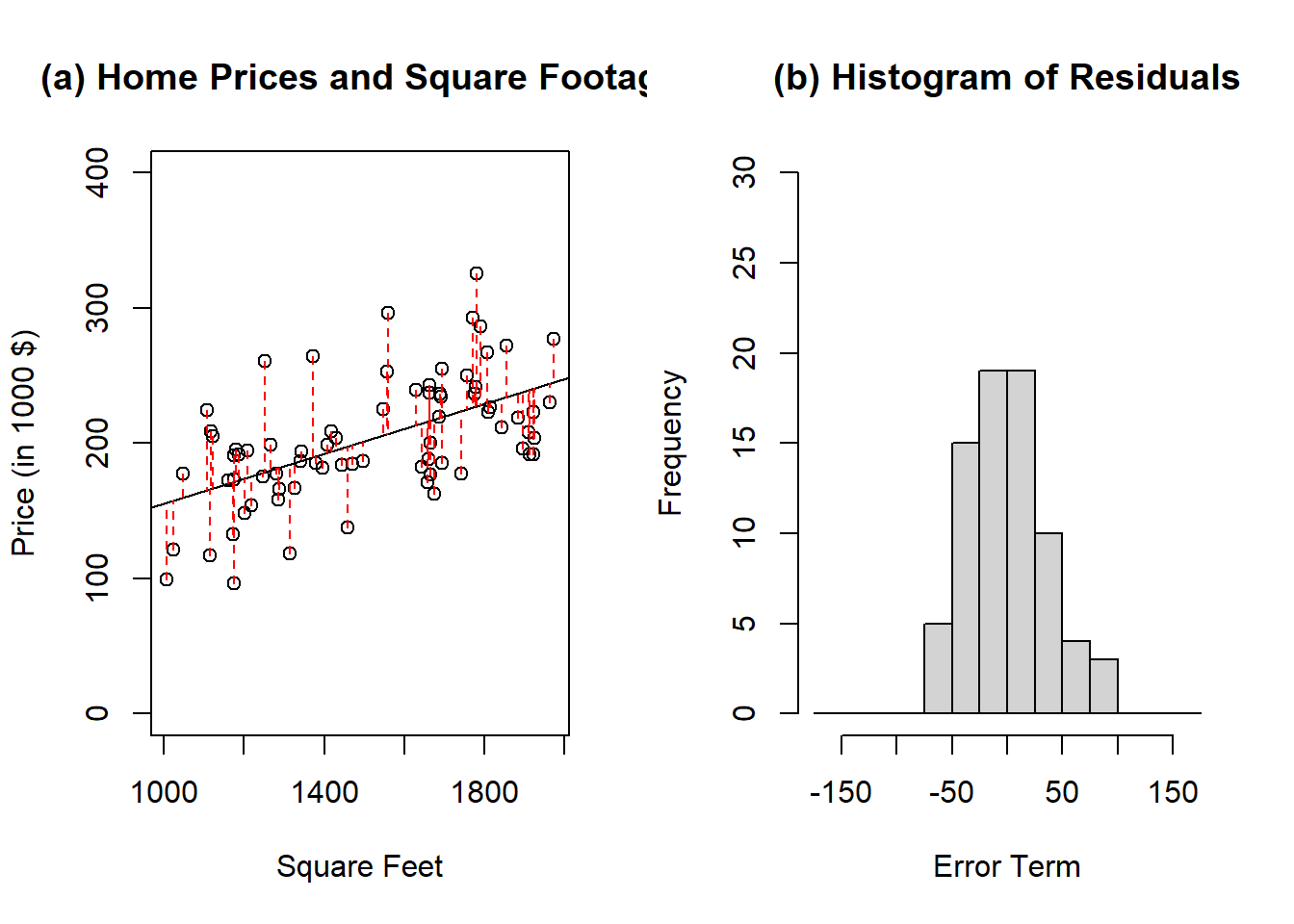
Figure 11.1: Example of regression line to model home values as a function of square footage. The red dashed lines in panel (a) represent the error terms associated with each observation. Panel (b) is the histogram associated with the error terms. The expected value of the error terms is zero and by assumption, the error terms are normally distributed.

The direction of the relationship is clear in the sense that the square footage (independent variable) influences the home value (dependent variable) and not vice versa. The red dashed lines are the vertical error terms. In the graph, the solid regression line is such that the sum of the squared error terms is minimized.

For the OLS Model to provide unbiased estimates, assumptions associated with the model are necessary. Later sections cover how to test if those assumptions are satisfied and how to correct the model if needed. The assumptions are:

• Linear in parameters, i.e., \(y_i = \beta_0 + \beta_1 x_i + \epsilon_i\). This does not assume a linear relationship between \(x\) and \(y\). Later chapters cover functional forms and how to model non-linear relationships with a linear model.
• The error terms have a zero mean, i.e., \(E(\epsilon_i)=0\).
• Homoscedasticity, i.e., \(Var(\epsilon_i) = \sigma^2\) (Figure \(\ref{fig:BVR_heteroscedasticity}\)).
• No autoregression, i.e., \(Cov(\epsilon_i,\epsilon_j)=0\).
• Exogeneity of the independent variable, i.e., \(E(\epsilon_i|x_i)=0\).

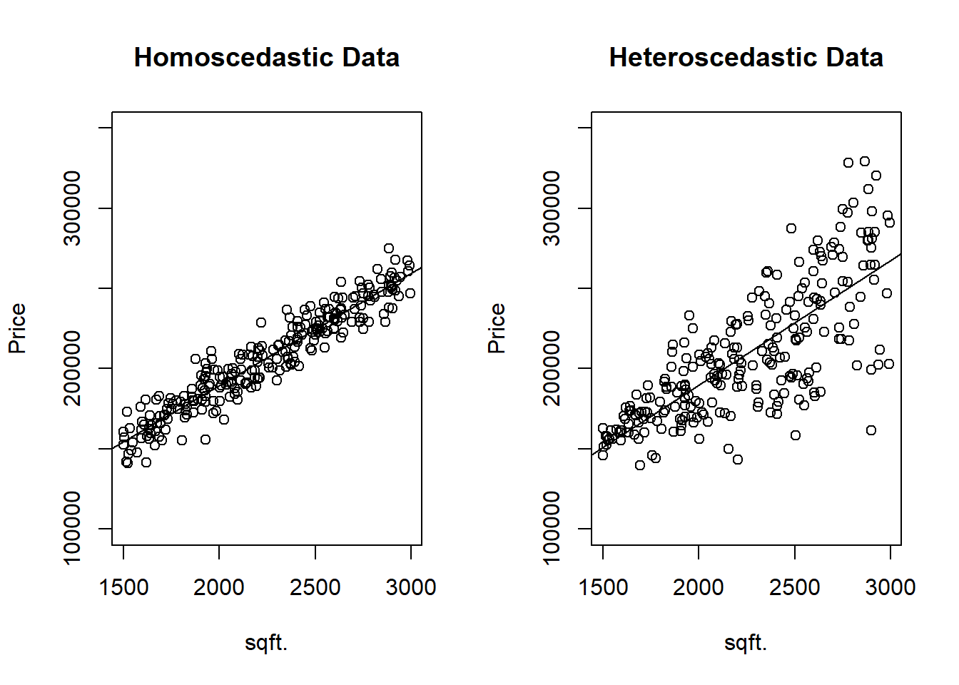
Figure 11.2: Panel (a) illustrates homoscedastic data whereas Panel (b) illustrates heteroscedastic data. The coefficient estimates will be unbiased by the standard error are larger for the model suffering from heteroscedasticity.