11.2 Hypothesis Testing

To determine whether there is a statistically significant relationship between the variables, a hypothesis test with respect to the coefficients \(\beta_0\) and \(\beta_1\) must be conducted. Every statistical software package provides this hypothesis test and no additional calculations are necessary. For the hypothesis test to be valid, the error terms must be normally distributed. Given this assumption, we are using the following \(t\)-statistic with \(n-2\) degrees of freedom. Note that the degrees of freedom decrease with every additional \(\beta\). This becomes relevant in the case of multivariate regression. The test statistic is

\[\frac{\hat{\beta}-\beta}{se_{\hat{\beta}}} \sim t_{n-2}\]

The test statistic for \(\beta_1\) can be written as

\[\frac{\hat{\beta}_1-\beta_1}{se_{\hat{\beta}_1}} \sim t_{n-2}\] where \[se_{\hat{\beta}_1} = \sqrt{\frac{\sum (y_i-\hat{y})^2 / (n-2) }{\sum(x_i-\bar{x})^2}}\] The existence of a linear relationship between \(X\) and \(Y\) can be tested with the above \(t\)-statistic by specifying H\(_0\): \(\beta_1 = 0\). Tests of hypotheses concerning \(\beta_0\) are much less frequent then tests concerning \(\beta_1\).

11.2.1 Numeric Example using Used Car Data

We are going to use a used car data set relating the price to the mileage of the car. Note that the direction of the relationship is clear, i.e., mileage affects price and not vice versa. The data can be found in the file . In R/RStudio, the regression can performed simply by the command .

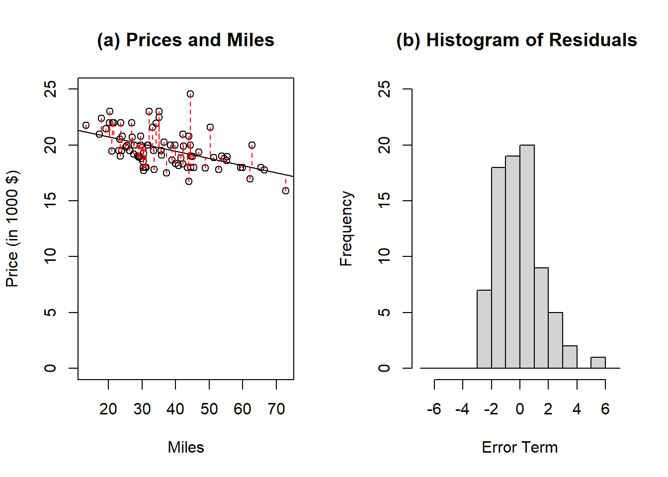
Figure 11.3: Example of regression line to model Honda prices as a function of miles. The red dashed lines in panel (a) represent the error terms associated with each observation. Panel (b) is the histogram associated with the error terms. The expected value of the error terms is zero and by assumption, the error terms are normally distributed.

In general, there are two problems with interpreting the intercept. First, if the range of \(x\) and \(y\) does not include the intercept then it is difficult to attach any meaning to the intercept. Second, the intercept can be negative although in reality, this could not be possible. In almost all regression models, we do not care about the intercept.

For the purpose of this example, we are using 25 observations and have divided the price and miles by 1000. Note that scaling the variables does not affect your statistical model in terms of significance.

Note that the average price is 18.963 and the average mileage is 38.922. Given the values above, we find that \(\beta_1 =-246.07/3844.44=-0.064\) and \(\beta_0 = 18.963 -(-0.064) \cdot 38.922 = 21.45\). For the goodness of fit measure \(R^2\), we have \[\begin{equation*} R^2 = 1-\frac{53.41}{69.16} = 0.2278 \end{equation*}\] And for the standard error of \(\beta_1\), we have \[\begin{equation*} se_{\hat{\beta}_1} = \sqrt{\frac{53.41/23}{3844.44}} = 0.02458 \end{equation*}\] Since we have the intercept and slope coefficient, the regression line can be written as \(price = 21.45-0.064 \cdot miles\). For example, having a car with 37.329 miles (in thousand), leads to \(21.45-0.064(37.329)=19.07\).