19.4 Autoregressive Model

An autoregressive model includes lagged dependent variables. One of the simplest model is an autoregressive model of order 1, i.e., an AR(1) Model \[y_t = \alpha + \beta \cdot y_{t-1} + \epsilon_t\] where \(\epsilon_t \sim N(0,\sigma^2)\). Consider the data of earthquakes over magnitude 7 in the data set quakes:

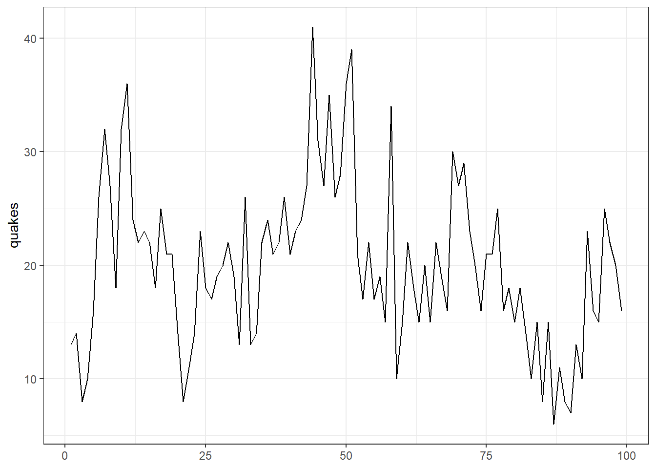
In a first step, a scatter plot is constructed of \(Y_{t-1}\) and \(y_t\). The easiest way is to use the function acf:

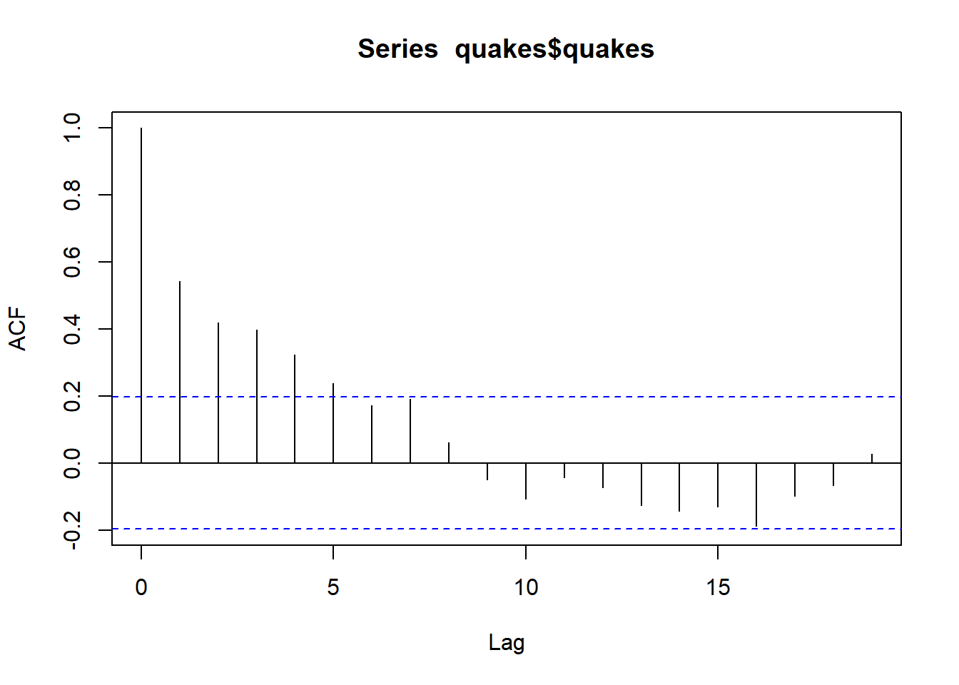
## [1] 0.5417329

The correlation coefficicent of 0.25 indicates a weak positive correlation between the number of earthquakes in periods \(t\) and \(t-1\). Remember that correlation is not causation. The AR(1) model can be estimated with the lm() function used previously:

summary(lm(quakes~Lag(quakes),data=quakes))

## 
## Call:
## lm(formula = quakes ~ Lag(quakes), data = quakes)
## 
## Residuals:
##     Min      1Q  Median      3Q     Max 
## -17.666  -3.901  -0.351   3.050  17.138 
## 
## Coefficients:
##             Estimate Std. Error t value Pr(>|t|)    
## (Intercept)  9.19070    1.81924   5.052 2.08e-06 ***
## Lag(quakes)  0.54339    0.08528   6.372 6.47e-09 ***
## ---
## Signif. codes:  0 '***' 0.001 '**' 0.01 '*' 0.05 '.' 0.1 ' ' 1
## 
## Residual standard error: 6.122 on 96 degrees of freedom
##   (1 observation deleted due to missingness)
## Multiple R-squared:  0.2972, Adjusted R-squared:  0.2899 
## F-statistic:  40.6 on 1 and 96 DF,  p-value: 6.471e-09

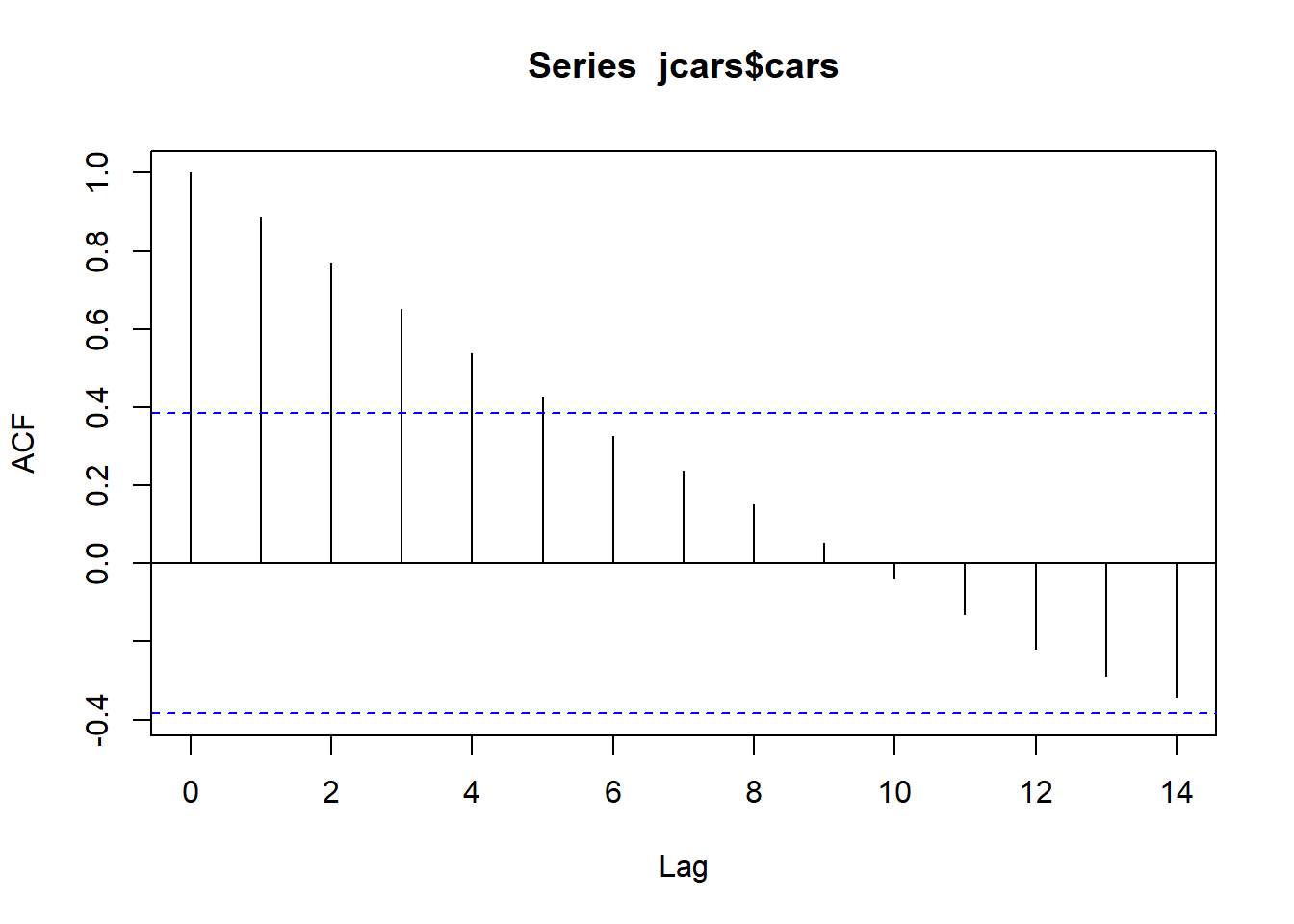
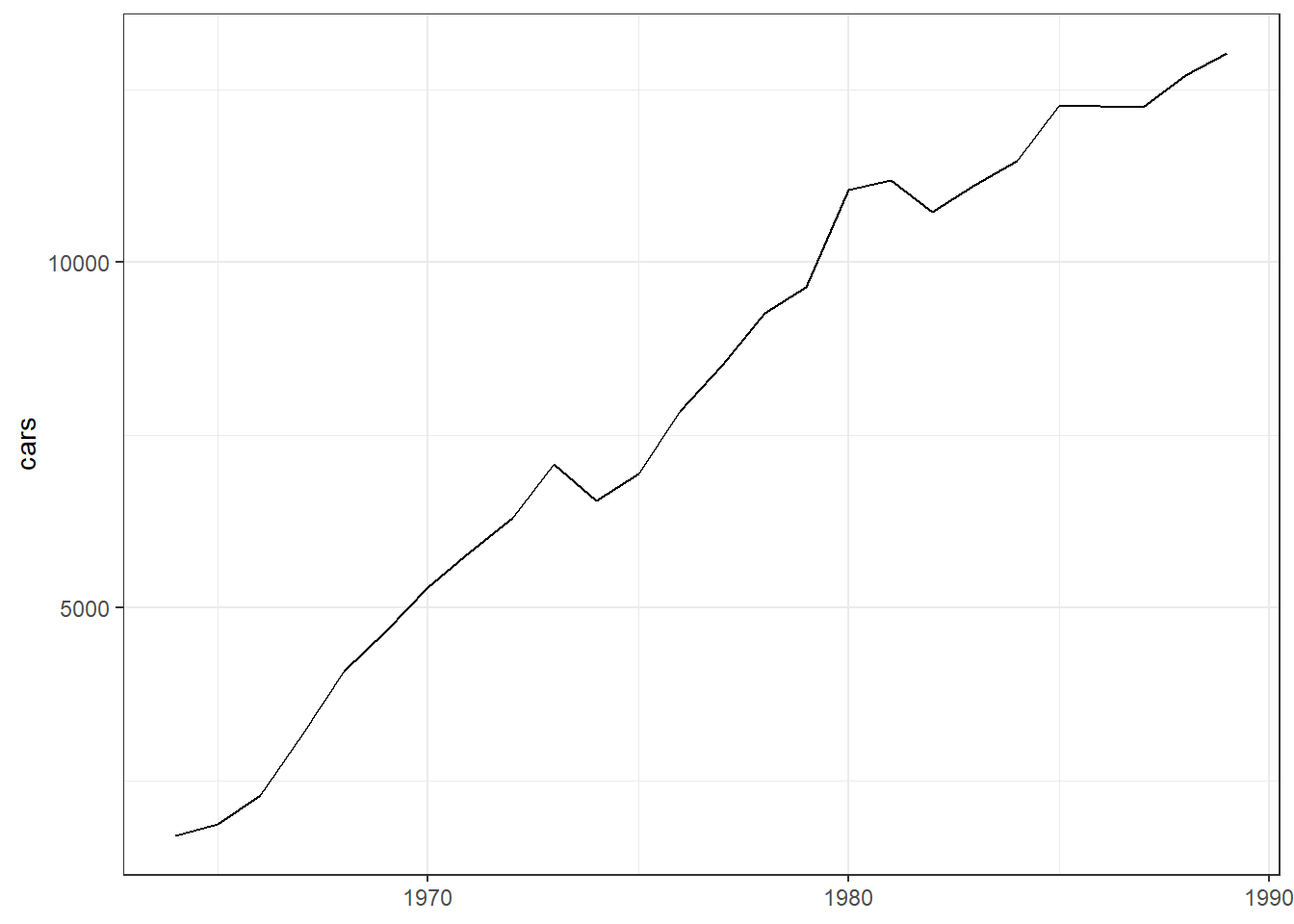
Note that although the slope coefficient associated with the lagged term is statistically significant, the R-squared value is very low. The third examples uses data on Japanese car production (jcars) to illustrate the concept of autocorrelation. The focus is on car production after 1963.

In a first step, the data is visualized using ggplot:

ggplot(jcars,aes(x=year,y=cars))+geom_line()+theme_bw()+theme(axis.title.x=element_blank())

The sample autocorrelation function (ACF) is the correlation between \(y_t\) and \(y_{t-1}\), \(y_{t-2}\), \(y_{t-3}\), and so on. It can be written as follows: \[\rho_j = \frac{Cov(y_t,y_{t-j})}{\sqrt{Var(y_t)\cdot Var(y_{t-j})}}\]

The ACF can be used to identify a possible structure of time series either of the actual time series or the residuals of the regression. The autocorrelation function (ACF) is plotted using the function acf() in R.

acf(jcars$cars)