4.2 Measures of Dispersion

The easiest measure of dispersion is called the range which is the largest value minus the smallest value in the data set. A measure used far more often is the variance. Think of the variance as a measure describing how far the data is spread around the mean. Recall from Chapter 1 that there we distinguish between a population and a sample. The population is characterized by unknown parameters and we use statistics based on sample to say something about the unknown population parameters. The distinction between population and sample is important regarding the variance. The population variance is calculated as follows: \[\sigma^2 = \frac{1}{N} \sum^N_{i=1}(x_i-\mu)^2\]

The sample variance is calculated as follows: \[s^2 = \frac{1}{N-1} \sum^N_{i=1}(x_i-\bar{x})^2\] The population variance is used to calculate the variance of the entire population. For example, if a professor is interested in calculating the variance associated with the final exam, they would use population variance equation because the class is not a sample of a larger population. The second equation dividing by $N-1$ is used if we have a sample and want to estimate (!) the variance associated with the population. Consider the figure below which illustrates the difference. A randomly generated data set contains 100,000 observations with $\mu=50$ and $\sigma=20$. An simulation procedure takes 1000 sample with sample sizes varying from 2 to 50 (horizontal axis). For each of the sample, the population variance is estimated by dividing by either $N$ or $N-1$. The estimates dividing by N-1 are closer to the population standard deviation than for the samples divided by N.

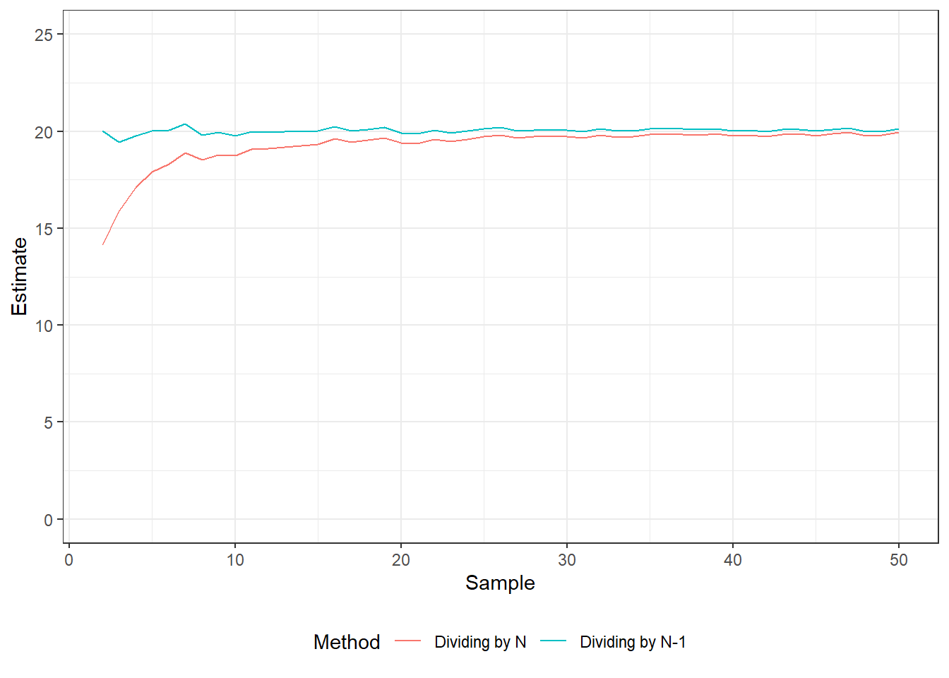
Figure 4.1: Difference between dividing by N and N-1 to estimate the variance.

The coefficient of variation standardizes the standard deviation $\sigma$ by the mean, i.e., $CV=\sigma/\mu$. Because the magnitude of the standard deviation depends on the mean, it is sometimes necessary to calculate the coefficient of variation to make two or more standard deviations comparable. For example, suppose you are comparing residential home values in California and Indiana. You calculate the mean and standard deviation for California as $2,000,000 and $400,000, respectively. The mean and standard deviation for Indiana are $125,000 and $50,000, respectively. Calculating the coefficient of variation ($CV$) for both states leads to $CV_{CA} = 0.2$ and $CV_{IN} = 0.4$. Hence, there is much more variation in the home values for Indiana than there is in California.