15 Binary Choice
There are slides and a YouTube Video associated with this chapter:
Binary choice models are part of a large class of so-called qualitative choice models which are used for qualitative dependent variables. Consider the following outcomes of interest:
- Is a person in the labor force?
- Will an individual vote yes on a particular issue?
- Did a person watch the last Super Bowl?
- Have you purchased a new car in the past year
- Did you do any charitable contributions in the past year?
- Did you vote during the last election?
- Does an individual recidivate after being released from prison?
For those questions, the dependent variable is either 0 (“no”) or 1 (“yes”). For binary choice models, the outcome is interpreted as a probability, i.e., what is the probability of a person to answer “yes” to those questions.
In the next chapter, the model is expanded to consider more than binary outcomes. Those models include categorical dependent variable that are either naturally ordered or have no ordering. Examples of naturally ordered categorical variables are:
- Level of happiness: Very happy, happy, ok, or sad.
- Intention to get a COIVID-19 vaccine: Definitely yes, probably yes, probably no, or definitely no
Two examples about categorical dependent variable which have no ordering are:
- Commute to campus: Bike, car, walk, or bus
- Voter registration: Democrat, Republican, or independent
For all those models, the outcome of interest is the probability to fall into a particular category. For binary choice models which are considered in this chapter, the outcome of interest is the probability to fall into the 1 (“yes”) category. For binary choice models, y takes one of two values: 0 or 1. And the model will specify \(Pr(y=1|x)\) where x are the independent variables.
Consider the decision to purchase organic food. Assume that you have data about the income of respondents as well as information if they purchase organic food. The purchase decision (“yes” or “no”) is on the vertical axis and the income is on the horizontal axis.
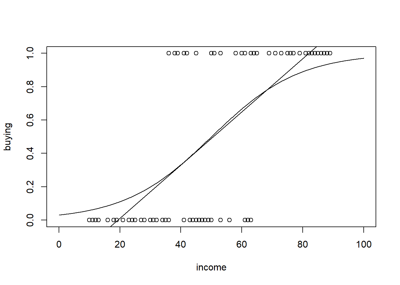
Remember that the probability has be bounded between 0 and 1. Hence, we need to find a function \(G(z)\) such that \(0 \leq G(z) \leq 1\) for all values of \(z\) and \(P(y=1|x)=G(z)\). Popular choices for \(G(z)\) are the cumulative normal distribution function (“Probit Model”) and the logistic function (“Logit Model”). For what follows, let \(z=\beta_0+\beta_1 \cdot x_1 + \cdots + \beta_k \cdot x_k\). For the probit model, \(G(z)\) is written as
\[Pr(y = 1) = G(z)=\Phi(z)\]
where \(\Phi\) represents the cumulative normal. And for the logit model, \(G(z)\) is written as
\[Pr(y = 1) = G(z)=\frac{e^z}{1+e^z}=\frac{1}{1+e^{-z}}\]
The interpretation of the logit and probit estimates is not as straightforward as in the multivariate regression case. In general, we care about the effect of \(x\) on \(P(y=1|x)\). The sign of the coefficient shows the direction of the change in probability. The approximation to the marginal effect if \(x\) is roughly continuous:
\[\Delta P(y=1|x) \approx g(\hat{\beta}_0 + x \cdot \hat{\beta}) \cdot \beta_j \cdot \Delta x_j\]
To obtain the marginal effects in R, an additional step is necessary. Let us illustrate the binary choice model using the data set organic and a logit model. The results of interest for the binary choice model are the (1) coefficient estimates, (2) marginal effects, and (3) predicted probabilities.