12.6 Exercises
Ohio Schools III (***): Consider the data sets
ohioincomeandohioscore. In a first step, merge the two data sets by IRN. For all questions below, interpret the coefficients in terms of direction, magnitude, and statistical significance.- Estimate the following equation and report the output. \[score = \beta_0 + \beta_1 \cdot medianincome + \beta_2 \cdot enrollment\]
- Estimate the following equation. Compare your answer to the previous part. Do the coefficients change in magnitude? How do you interpret the squared term? \[score = \beta_0 + \beta_1 \cdot medianincome + \beta_2 \cdot enrollment + \beta_3 \cdot medianincome^2\]
Honda vs. BMW (***): The data sets
hondaandbmwcontain prices and mileage of used Honda and BMW cars in the Indianapolis area. For BMW, you have a dummy variable which indicates all-wheel drive (\(allwheeldrive\) = 1) or rear-wheel drive (\(allwheeldrive\) = 0).- Run a regression with price as the dependent variable and miles as the independent variable for both cars (separately). Report the intercept and slope coefficients. Interpret your results, e.g., how does an increase in miles affect the price of the cars.
- Generate two scatter plots of the data and the fitted lines. For each car, I want the scatter plot and the fitted line in the same graph. What can you say about the difference in depreciation of the two cars.
WDI (**): Using the data in
wdi, estimate the equation below for the year 2018. Report and interpret the results: \[fertrate = \beta_0 + \beta_1 \cdot gdp+ \beta_2 \cdot litrate\]Retail (***): This exercise will demonstrate the use of dummy variables to model so-called seasonality in the data
retail. Note that time series analysis is a fairly complex topic and this question only serves as an introduction. Using the data inretail, estimate the following regression model: \[retail = \beta_0 + \beta_1 \cdot t + \sum_{m=1}^{11} \beta_m \cdot D_m\] where \(t\) represents a simple time trend and \(D_m\) are monthly dummy variables. Make sure to only include 11(!) monthly dummy variables. Is there seasonality in the data? Interpret.Indy Homes I (***): The data
indyhomescontains home values of two ZIP codes in Indianapolis. In this exercise, you will estimate the value of homes (dependent variable) based on a set of independent variables. The variables are mostly self-explanatory. The variables \(levels\) and garage refers to the number of \(stories\) and the garage parking spots, respectively.- Create a dummy variable called \(northwest\) for the 46268 ZIP code.
- Report the results of the following regression equation \[\ln(price)=\beta_0+\beta_1 \cdot \ln(sqft)+\beta_2 \cdot northwest+\beta_3 \cdot \ln(lot)+\beta_4 \cdot bed+\beta_5 \cdot garage\\ + \beta_6 \cdot levels+ \beta_7 \cdot northwest \cdot levels\]
- Interpret each coefficient from the previous part and how it affects \(ln(price)\). How do you interpret the interaction term?
- What is the expected home value of a house in the 46228 ZIP code area with the following characteristics: 1800 sqft, 0.54 acres lot, 4 bedrooms, 3 bathrooms, 2 garage spots, and 1 story.
Pork Demand (***): In this exercise, you will estimate the per-capita pork demand as a function of pork prices and the prices of substitutes (beef and chicken) as well as real disposable income. Use the date
meatdemandfor this exercise. Estimate the following equation and interpret the coefficients. Are the signs of the coefficients what you would expect? \[\ln(q_{pork}) = \beta_0 + \beta_1 \cdot \ln(p_{pork}) + \beta_2 \cdot \ln(p_{chicken}) + \beta_3 \cdot \ln(p_{beef}) + \beta_4 \cdot \ln(rdi)\]NFL I (***): This question will have you create a similar analysis to the one found in Berri et al. (2011). The corresponding data is in
nfl: \[\ln(total)=\beta_0+\beta_1 \cdot yards+\beta_2 \cdot att+\beta_3 \cdot exp+\beta_4 \cdot exp^2 \\ +\beta_5 \cdot draft1+\beta_6 \cdot draft2+\beta_7 \cdot veteran+\beta_8 \cdot changeteam \\+\beta_9 \cdot pbowlever+\beta_{10} \cdot symm\] Report the output and interpret the coefficients in terms of statistical significance and direction (i.e., sign).Boston (***): For this exercise, use the data set
boston. In a first step, execute the following code:
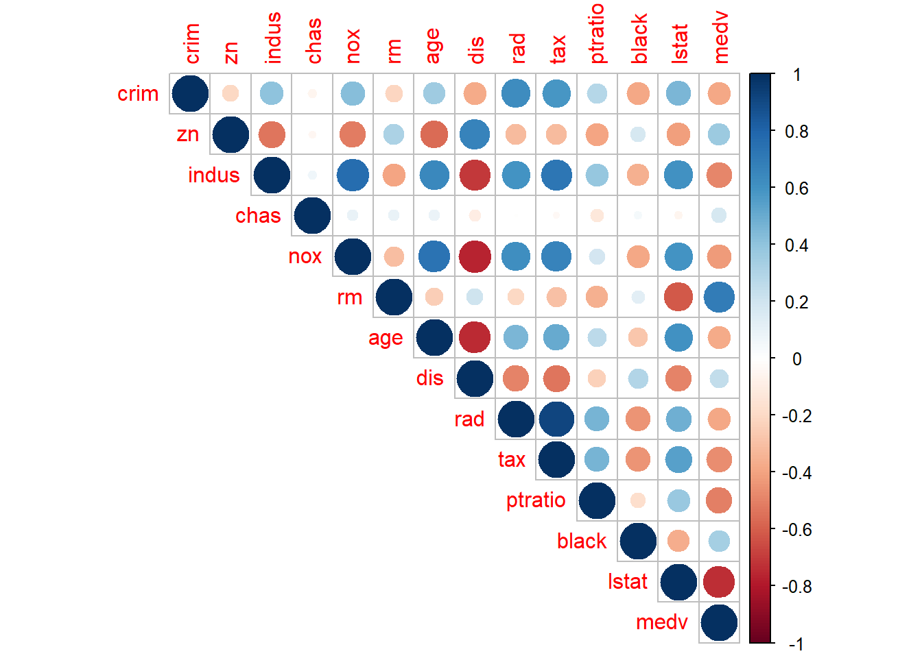
What does the resulting plot represent? In a second step, estimate the following model: \[medv = \beta_0 + \beta_1 \cdot lstat+ \beta_2 \cdot crim + \beta_3 \cdot age\]
Explain what exactly you estimated and what hypotheses are underlying the model. Lastly, estimate the model including all remaining independent variables. Are any of the results surprising?
BLM I (***): The following question is based on the article Black Lives Matter: Evidence that Police-Caused Deaths Predict Protest Activity. Note that we use a simplified version of the data set for this question. The dependent variable for this exercise is protest frequency (\(totprotests\)) and the independent variables are city population (\(pop\)), population density (\(popdensity\)), percent Black (\(percentblack\)), black poverty rate (\(blackpovertyrate\)), percent of population with at least a bachelor (\(percentbachelor\)), college enrollment (\(collegeenrollpc\)), share of democrats (\(demshare\)), and black police-caused deaths per 10,000 people (\(deathsblackpc\)). Interpret the output.
Furnished Apartments (***): Long-term furnished apartments are usually managed by companies. Some of those companies are more expensive than others. The dependent variable is \(rent\). Estimate a regression model using all other columns as independent variables. Which companies are more expensive than others and by how much? Is there a difference between living in Berlin (city) or one of its close suburbs (Potsdam). On a side note, people in Potsdam prefer the city not to be called a suburb since it is fairly sizable state capital.
U.S. Labor Market (***): Understanding wage determinants is essential for policymakers working on labor market policies. In this exercise, you will analyze the factors affecting individual wages, including education, experience, gender, and union membership using the data set
wagesfrom the Ecdat package. Estimate a multiple linear regression model where the dependent variable is \(wage\) (hourly wage), and the independent variables include \(education\) (years of schooling), \(experience\) (years of labor market experience), \(gender\) (female dummy variable: 1 for female, 0 for male), and \(union\) (union dummy variable: 1 for union member, 0 otherwise). Interpret the coefficient estimates regarding the effects of education and union membership on wages. Is there a significant gender wage gap after controlling for education and experience? Test for interaction effects between gender and education. Does the return to education differ between men and women?Dry January (***): The data set
djcontains the real per-capita retail sales of alcoholic beverages. Estimate a simple model including a time trend, dummy variables for the months, and a dummy variable indicating the beginning of the pandemic in the United States. For that date, I suggest to use April 2020. Interpret your results. Based on the data, how would you estimate the effects of Dry January? That is, the movement which started in 2014 to abstain from alcohol in January.