4.3 Histograms
In almost all cases, a visual inspection of the data is appropriate. Although numerical statistics such as mean and/or standard deviation exist, many fail to easily identify patterns or anomalies. Histograms are probably the most basic method to graphically summarize data and are also good approximations of the probability distributions. Suppose you have a data set \(x_1,x_2, \dots, x_n\). You divide the range of values into bins. For example, if a data set ranges from 75 to 155, then a possible bin size could be 10, i.e., 75, 85,…, 155. The height of the bar for each bin is determined by the number of observations in the bin range. Those bins usually have the same size but it is not necessary. Consider the eruption and waiting times of Old Faithful geyser in Yellowstone National Park. Panel (a) and (b) represent the histograms of eruption and waiting time, respectively.
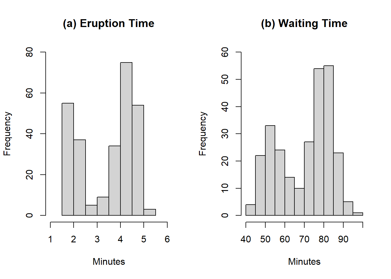
Figure 4.2: Histogram of eruption and waiting time of Old Faithful geyser
To draw a histogram of the data as shown in the above figure, use the folling command:
hist(faithful$eruptions)
Note that you can control the appearance of the histogram by using options:
hist(faithful$eruptions,main="Eruption",xlab="Minutes",xlim=c(1,6),ylim=c(0,80))