19.7 Forecasting Japanense Car Production

Model 1: Regular OLS Model \[y_t = \beta_0 + \beta_1 t + \epsilon_t\] Model 2: Autoregressive Model \[ y_t = \beta_0 + \beta_1 t + n_t \quad \text{where} \quad n_t = \phi_1 n_{t-1} + \epsilon_t\]

summary(lm(cars~year,data=jcars))

## 
## Call:
## lm(formula = cars ~ year, data = jcars)
## 
## Residuals:
##     Min      1Q  Median      3Q     Max 
## -911.62 -406.49   47.09  353.35 1351.64 
## 
## Coefficients:
##               Estimate Std. Error t value Pr(>|t|)    
## (Intercept) -924484.82   30143.45  -30.67   <2e-16 ***
## year            471.81      15.25   30.94   <2e-16 ***
## ---
## Signif. codes:  0 '***' 0.001 '**' 0.01 '*' 0.05 '.' 0.1 ' ' 1
## 
## Residual standard error: 583.2 on 24 degrees of freedom
## Multiple R-squared:  0.9755, Adjusted R-squared:  0.9745 
## F-statistic: 957.1 on 1 and 24 DF,  p-value: < 2.2e-16

auto.arima(jcars$cars)

## Series: jcars$cars 
## ARIMA(0,1,0) with drift 
## 
## Coefficients:
##          drift
##       452.9600
## s.e.   83.6424
## 
## sigma^2 = 182188:  log likelihood = -186.37
## AIC=376.75   AICc=377.29   BIC=379.18

bhat = Arima(jcars$cars,order=c(1,0,0),include.constant=TRUE,include.drift = TRUE)
summary(bhat)

## Series: jcars$cars 
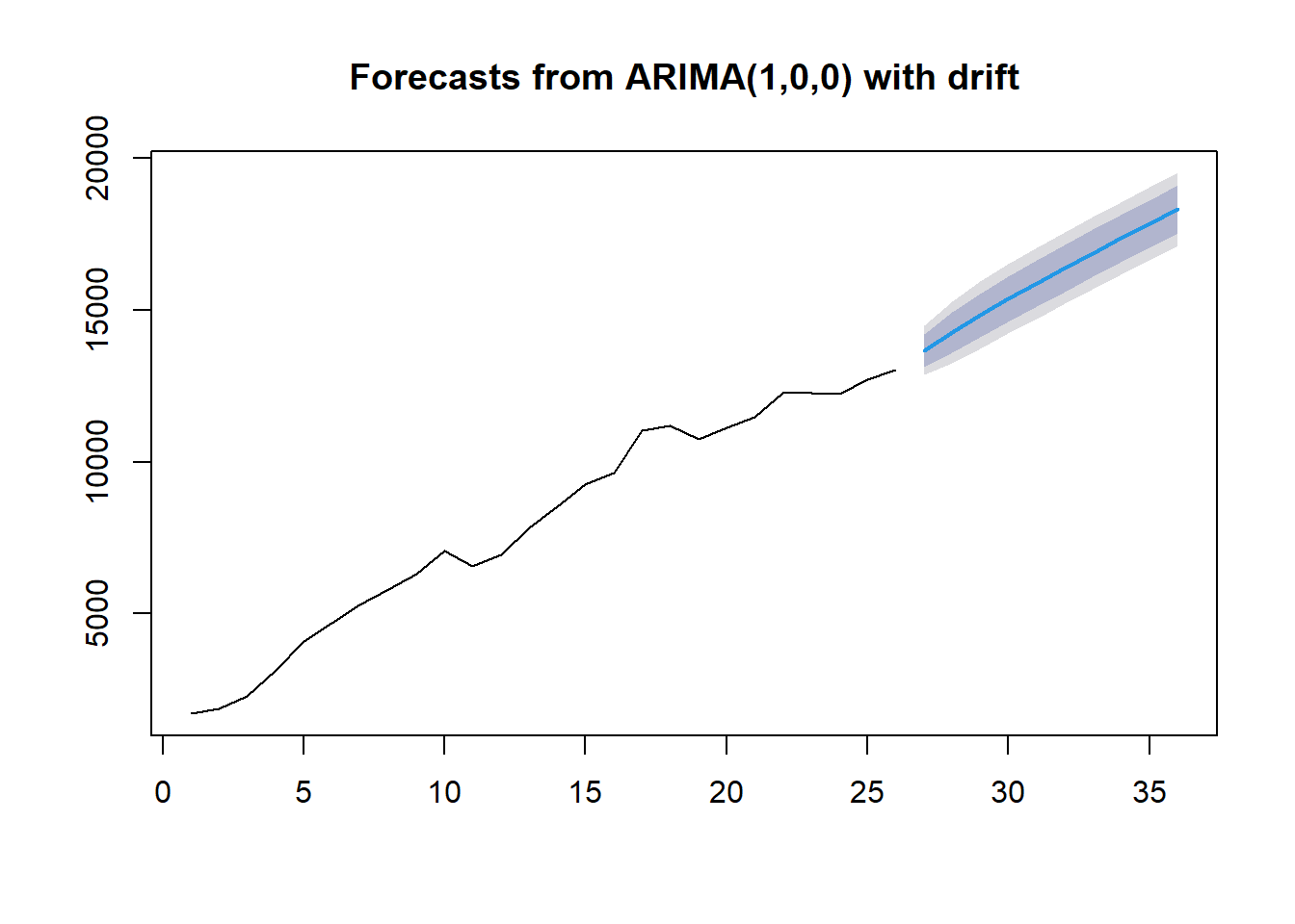
## ARIMA(1,0,0) with drift 
## 
## Coefficients:
##          ar1  intercept     drift
##       0.7363  1662.4148  463.5637
## s.e.  0.1347   471.7223   29.2265
## 
## sigma^2 = 171700:  log likelihood = -192.38
## AIC=392.77   AICc=394.67   BIC=397.8
## 
## Training set error measures:
##                    ME     RMSE      MAE        MPE     MAPE      MASE      ACF1
## Training set 17.28081 389.7285 311.2957 -0.7522648 5.354775 0.5840007 0.1564618

plot(forecast(bhat))