11.4 About the Importance of the Assumptions
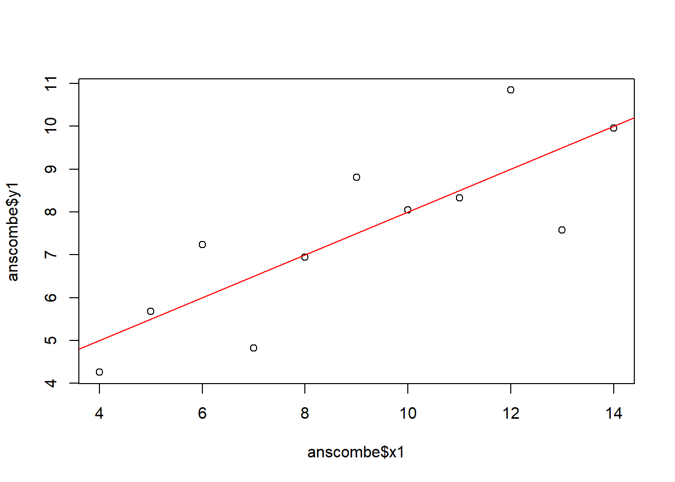
The data in anscombe illustrates the danger of simply relying on the regression output. The so-called Anscombe’s Quartet includes \(i=1,\dots,4\) data series denoted \(y_i\) (dependent variable) and \(x_i\) (independent variable). Estimate the four regression models and compare the results and the conclusions you draw from the output. Next, plot the observations and include the fitted line. The regression output for the first set:
##
## Call:
## lm(formula = y1 ~ x1, data = anscombe)
##
## Residuals:
##      Min       1Q   Median       3Q      Max
## -1.92127 -0.45577 -0.04136  0.70941  1.83882
##
## Coefficients:
##             Estimate Std. Error t value Pr(>|t|)
## (Intercept)   3.0001     1.1247   2.667  0.02573 *
## x1            0.5001     0.1179   4.241  0.00217 **
## ---
## Signif. codes:  0 '***' 0.001 '**' 0.01 '*' 0.05 '.' 0.1 ' ' 1
##
## Residual standard error: 1.237 on 9 degrees of freedom
## Multiple R-squared:  0.6665, Adjusted R-squared:  0.6295
## F-statistic: 17.99 on 1 and 9 DF,  p-value: 0.00217
And the associated scatter plot with the regression equation: