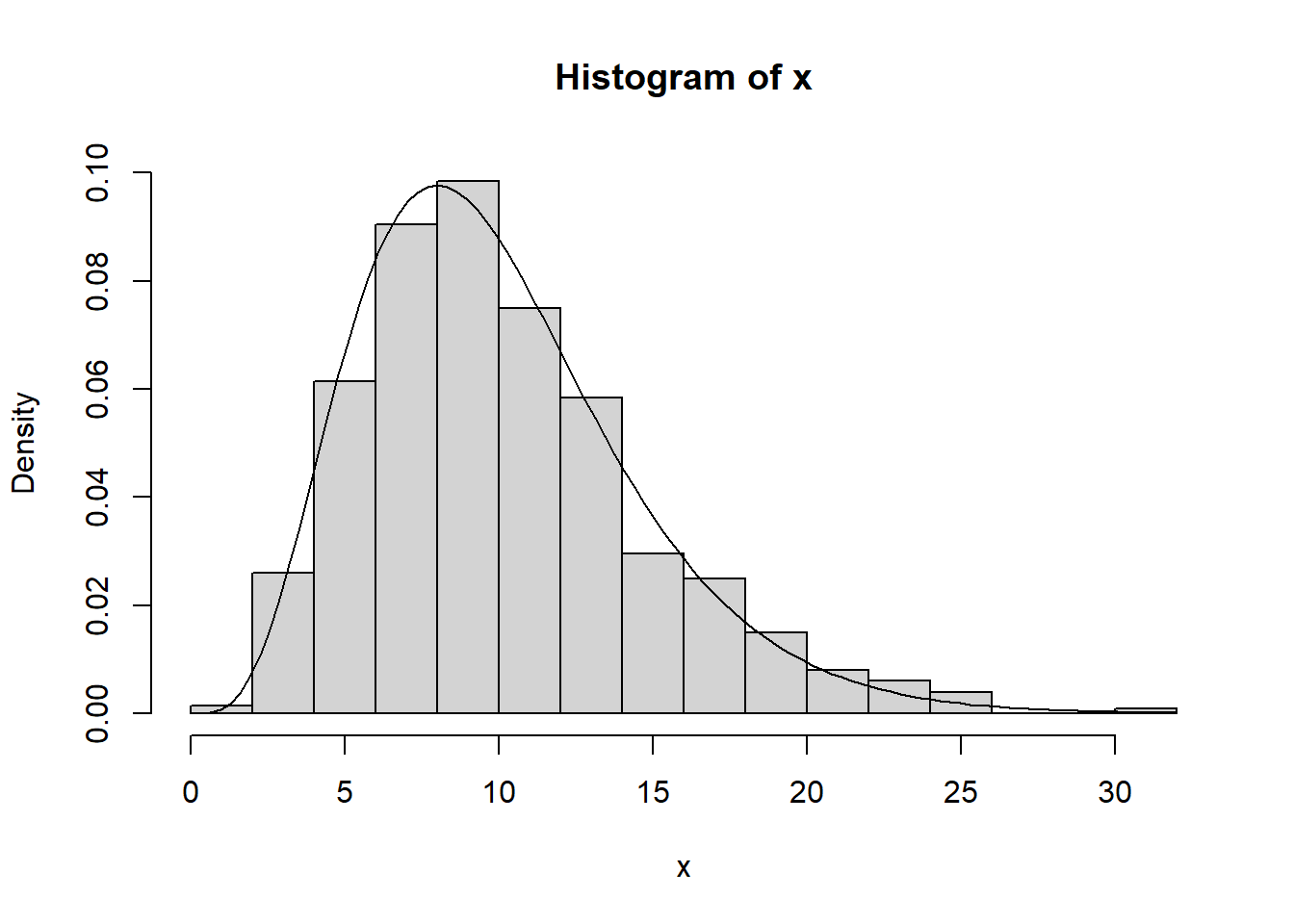
10.1 Chi-Square Test (\(\chi^2\)-Test)
The \(\chi^2\)-test is used to conduct a hypothesis test on qualitative variables. Before introducing the procedure, a presentation of the \(\chi^2\)-distribution is necessary.
Given the values \(Z_1, Z_2, \dots , Z_k\) independently drawn from standard normal distribution, then the squared sum of those values follows a \(\chi^2\)-distribution: \[\sum_{i=1}^k Z_i^2 = Z \sim \chi^2_k\] where \(k\) specifies the degrees of freedom.

To conduct the hypothesis test, consider the data on voting and education in gss. Using the function CrossTable associated with the package gmodels, the following table can be constructed.
df        = subset(gss,vote20 %in% c(1,2) & degree %in% c(0:4),select=c("vote20","degree"))
CrossTable(df$degree,df$vote20,prop.r = FALSE,prop.c = FALSE,prop.chisq = FALSE,prop.t=FALSE)
##
##
## Cell Contents
## |-------------------------|
## | N |
## |-------------------------|
##
##
## Total Observations in Table: 3155
##
##
## | df$vote20
## df$degree | 1 | 2 | Row Total |
## -------------|-----------|-----------|-----------|
## 0 | 134 | 132 | 266 |
## -------------|-----------|-----------|-----------|
## 1 | 1054 | 399 | 1453 |
## -------------|-----------|-----------|-----------|
## 2 | 246 | 47 | 293 |
## -------------|-----------|-----------|-----------|
## 3 | 635 | 63 | 698 |
## -------------|-----------|-----------|-----------|
## 4 | 405 | 40 | 445 |
## -------------|-----------|-----------|-----------|
## Column Total | 2474 | 681 | 3155 |
## -------------|-----------|-----------|-----------|
##
## This table is similar to what has been presented previously except that all proportions have been removed and only the counts are presented. This is a 5-by-2 contingency table (the total columns are not considered part of the table). The variable education is less than high school (0), high school (1), junior college (2), bachelor (3), and graduate (4). Assuming independence, the expected value \(E\) for each cell is \[E=\frac{(\text{total of row})\cdot(\text{total of column})}{\text{total count}}\] For example, consider the cell “high school” and “voting” which contains 214 counts. The expected value under the null hypothesis that voting behavior is independent of education leads to the following: \[E_{1,1}=\frac{367 \cdot 518}{772} = 246.2513\] Those calculations can be conducted for each cell. Then, then the \(\chi^2\)-test statistic is calcualted as follows: \[\chi^2 = \sum_{i=1}^{r \cdot c} \frac{(O_i-E_i)^2}{E_i}\] where \(r \cdot c\) is number of rows multiplied by the number of colunms, \(O_i\) and \(E_i\) are the observed and exepected count in a cell, respectively. The degrees of freedom are calcualted as \((r-1)\cdot(c-1)\). Of course, instead of doing it manually, the following command can be used:
##
##  Pearson's Chi-squared test
##
## data:  df$degree and df$vote20
## X-squared = 265.27, df = 4, p-value < 2.2e-16
Due to the p-value being very small, we reject the hypothesis of independence. The \(\chi^2\) hypothesis test should only be used for qualitative data. For example, do not categorize income into quartiles to conduct a hypothesis test on whether voting depends on income.
The example of a 2-by-2 table is a special case
votegun   = subset(gss,
                   vote20 %in% c(1,2) &
                   owngun %in% c(1,2),
                   select = c("vote20","owngun"))
votegun$vote20 = ifelse(votegun$vote20==1,1,0)
votegun$owngun = ifelse(votegun$owngun==1,1,0)
t.test(votegun$vote20~votegun$owngun)
##
## Welch Two Sample t-test
##
## data: votegun$vote20 by votegun$owngun
## t = -4.2686, df = 1637.9, p-value = 2.08e-05
## alternative hypothesis: true difference in means between group 0 and group 1 is not equal to 0
## 95 percent confidence interval:
## -0.11603883 -0.04297346
## sample estimates:
## mean in group 0 mean in group 1
## 0.7474981 0.8270042##
## Pearson's Chi-squared test with Yates' continuity correction
##
## data: votegun$vote20 and votegun$owngun
## X-squared = 16.236, df = 1, p-value = 5.592e-05CrossTable(votegun$vote20,votegun$owngun,prop.r = FALSE,prop.c = FALSE,prop.chisq = FALSE,prop.t=FALSE)##
##
## Cell Contents
## |-------------------------|
## | N |
## |-------------------------|
##
##
## Total Observations in Table: 2010
##
##
## | votegun$owngun
## votegun$vote20 | 0 | 1 | Row Total |
## ---------------|-----------|-----------|-----------|
## 0 | 328 | 123 | 451 |
## ---------------|-----------|-----------|-----------|
## 1 | 971 | 588 | 1559 |
## ---------------|-----------|-----------|-----------|
## Column Total | 1299 | 711 | 2010 |
## ---------------|-----------|-----------|-----------|
##
##