17.2 Censoring
In the case of censoring, the values of the dependent variable are reported at a certain point if they are above or below a certain value.
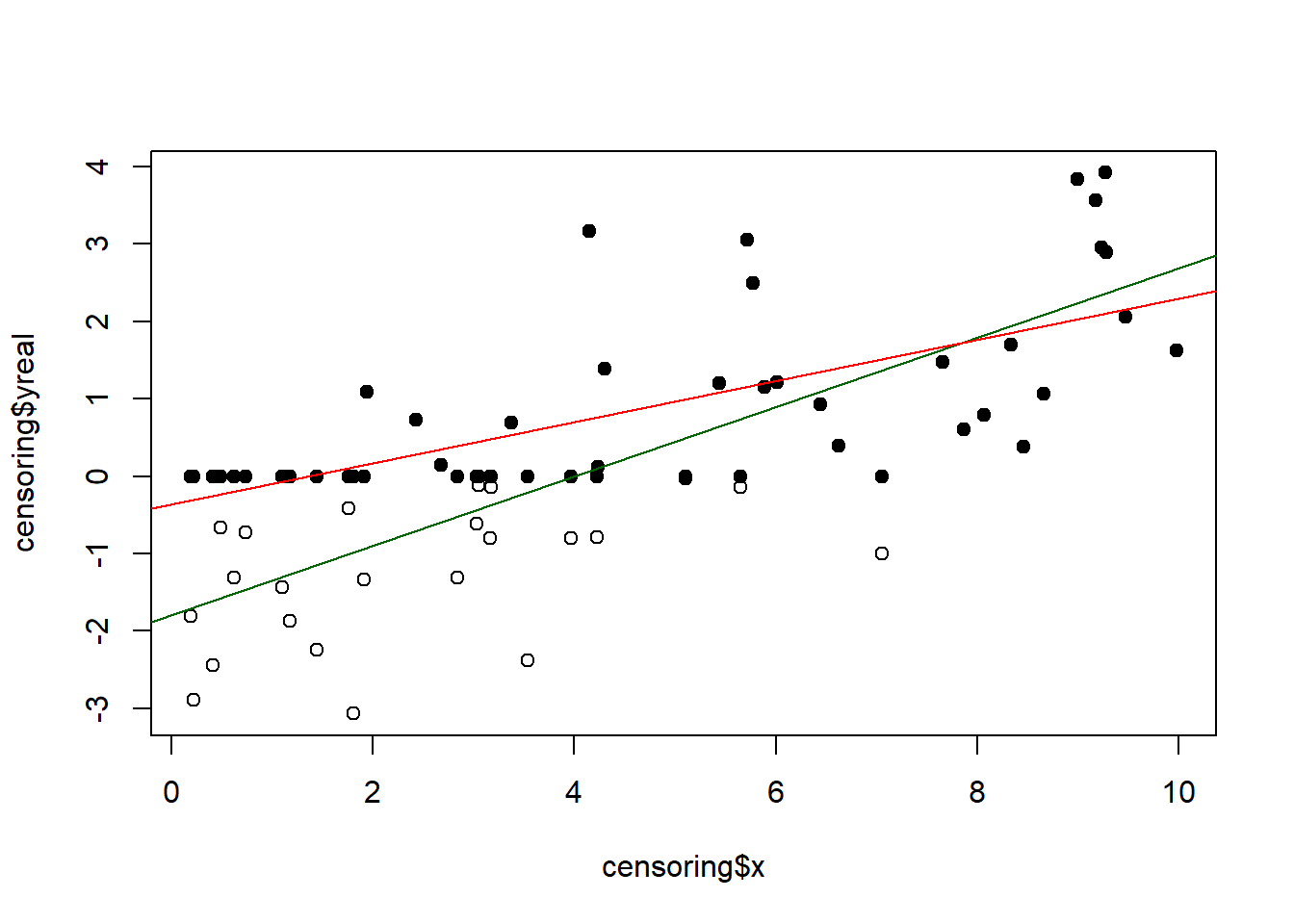
If all data was reported at the correct value, the following following regression model could be executed:
##
## Call:
## lm(formula = yreal ~ x, data = censoring)
##
## Residuals:
##      Min       1Q   Median       3Q      Max
## -2.60012 -0.59843  0.00981  0.78105  2.05397
##
## Coefficients:
##             Estimate Std. Error t value Pr(>|t|)
## (Intercept) -2.25290    0.27739  -8.122 1.44e-10 ***
## x            0.52603    0.04888  10.762 2.17e-14 ***
## ---
## Signif. codes:  0 '***' 0.001 '**' 0.01 '*' 0.05 '.' 0.1 ' ' 1
##
## Residual standard error: 0.951 on 48 degrees of freedom
## Multiple R-squared:  0.707,  Adjusted R-squared:  0.7009
## F-statistic: 115.8 on 1 and 48 DF,  p-value: 2.169e-14
Ignoring censoring leads to biased results:
##
## Call:
## lm(formula = y ~ x, data = censoring)
##
## Residuals:
##      Min       1Q   Median       3Q      Max
## -0.94411 -0.51345  0.03089  0.37886  1.25169
##
## Coefficients:
##             Estimate Std. Error t value Pr(>|t|)
## (Intercept) -0.54026    0.17443  -3.097  0.00326 **
## x            0.29534    0.03074   9.608 9.21e-13 ***
## ---
## Signif. codes:  0 '***' 0.001 '**' 0.01 '*' 0.05 '.' 0.1 ' ' 1
##
## Residual standard error: 0.5981 on 48 degrees of freedom
## Multiple R-squared:  0.6579, Adjusted R-squared:  0.6508
## F-statistic: 92.32 on 1 and 48 DF,  p-value: 9.212e-13
Using the R package censReg) allows for the reduction of the bias:
##
## Call:
## censReg(formula = y ~ x, data = censoring)
##
## Observations:
##          Total  Left-censored     Uncensored Right-censored
##             50             17             33              0
##
## Coefficients:
##             Estimate Std. error t value Pr(> t)
## (Intercept) -1.41227    0.29576  -4.775 1.8e-06 ***
## x            0.41466    0.04717   8.791 < 2e-16 ***
## logSigma    -0.33824    0.12631  -2.678 0.00741 **
## ---
## Signif. codes:  0 '***' 0.001 '**' 0.01 '*' 0.05 '.' 0.1 ' ' 1
##
## Newton-Raphson maximisation, 6 iterations
## Return code 1: gradient close to zero (gradtol)
## Log-likelihood: -44.496 on 3 Df