12.1 Introduction

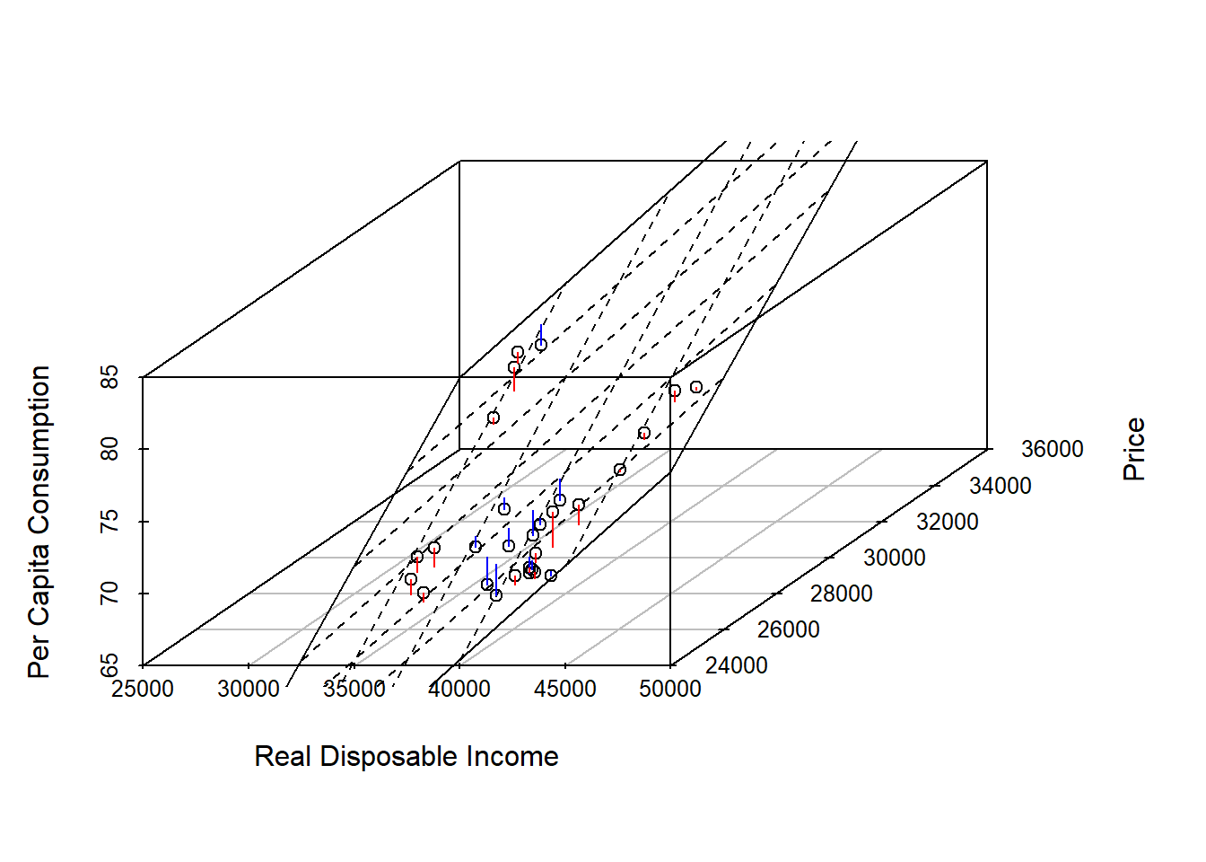
Recall the bivariate regression model with one independent and one dependent variable: \[y=\beta_0+\beta_1 \cdot x_1+\epsilon\] The multivariate linear regression model includes more than one independent variable and is simply an extension of the bivariate regression model: \[y=\beta_0+\beta_1 \cdot x_1+\beta_2 \cdot x_2 + \dots + \beta_k \cdot x_k + \epsilon\] Whether we consider the bivariate or multivariate model, the objective is always to minimize the sum of squared errors which has led to the name ordinary least square (OLS) model. The equation of a line can be determined using slope (\(\beta_0\)) and the intercept (\(\beta1\)), i.e.: \[E(y|x_1)=\beta_0+\beta_1 \cdot x_1\] The case of a regression model with two independent variable can still be represented in a 3-dimensional graph as depicted below

The purpose of the multivariate regression model is to measure the effect of independent variables on the dependent variable. It is crucial to control for everything else that could influence the dependent variable. For example, measuring the weekly grocery bill as a function of years of education might give you a statistically significant effect for education but if income is included, the effect for education might (most likely) disappear.

The first example involves estimating home values based on square footage and number of garage spots of a house in the 46268 ZIP code in Indianapolis. The data is contained in indyhomes.

indyhomes46268 = subset(indyhomes,zip==46268)
bhat = lm(price~sqft+garage,data=indyhomes46268)
summary(bhat)

## 
## Call:
## lm(formula = price ~ sqft + garage, data = indyhomes46268)
## 
## Residuals:
##    Min     1Q Median     3Q    Max 
## -58780  -7817   1582   7886  51803 
## 
## Coefficients:
##              Estimate Std. Error t value Pr(>|t|)    
## (Intercept) 81733.141  15896.004   5.142 5.20e-06 ***
## sqft           40.897      4.383   9.331 2.85e-12 ***
## garage      16580.964   7136.866   2.323   0.0245 *  
## ---
## Signif. codes:  0 '***' 0.001 '**' 0.01 '*' 0.05 '.' 0.1 ' ' 1
## 
## Residual standard error: 20710 on 47 degrees of freedom
## Multiple R-squared:  0.675,  Adjusted R-squared:  0.6611 
## F-statistic:  48.8 on 2 and 47 DF,  p-value: 3.388e-12

Depending on the nature of the variables, it might be necessary to scale your variables for ease of interpretation. This might be necessary if coefficients are very large or very small. A rescaling, e.g., dividing income by 1000, does affect the coefficients and the standard errors but has no effect on the t-statistics.